One of my jobs at Bang & Olufsen is to do the final measurements on each bespoke Beogram 4000c turntable before it’s sent to the customer. Those measurements include checking the end-to-end magnitude response, playing from a vinyl record with a sine sweep on it (one per channel), recording that from the turntable’s line-level output, and analysing it to make sure that it’s as expected. Part of that analysis is to very that the magnitude responses of the left and right channel outputs are the same (or, same enough… it’s analogue, a world where nothing is perfect…)
Today, I was surprised to see this result on a turntable that was being inspected part-way through its restoration process :
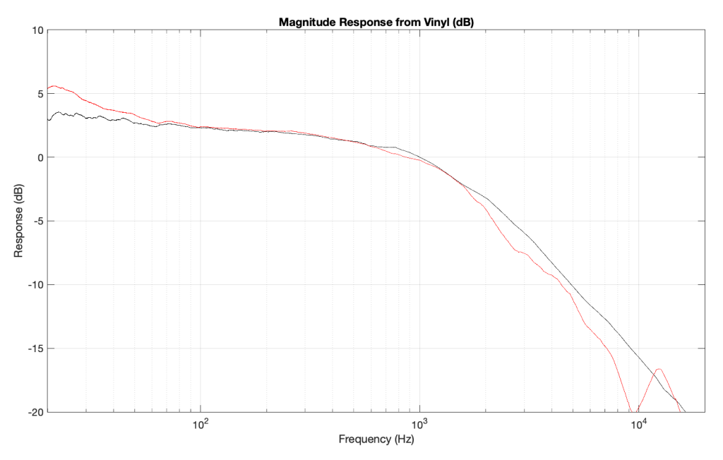
Taken at face value, this should have resulted in a rejection – or at least some very serious questions. This is a terrible result, with unacceptable differences in output level between the two channels. When I looked at the raw measurements, I could easily see that the left channel was behaving – it was the right channel that was all over the place.
The black curve looks very much like what I would expect to see. This is the result of playing a track that is a sine sweep from 20 Hz to 20 kHz, where the signal below 1 kHz follows the RIAA curve, whereas the signal above 1 kHz does not. This is why, after it’s been filtered using a RIAA preamp, the low frequency portion has a flat response, but the upper frequency band rolls off (following the RIAA curve).
Notice that the right channel (the red curve) is a mess…
A quick inspection revealed what might have been the problem: a small ball of fluff collected around the stylus. (This was a pickup that was being used to verify that the turntable was behaving through the restoration – not the one intended for the final customer – and so had been used multiple times on multiple turntables.)
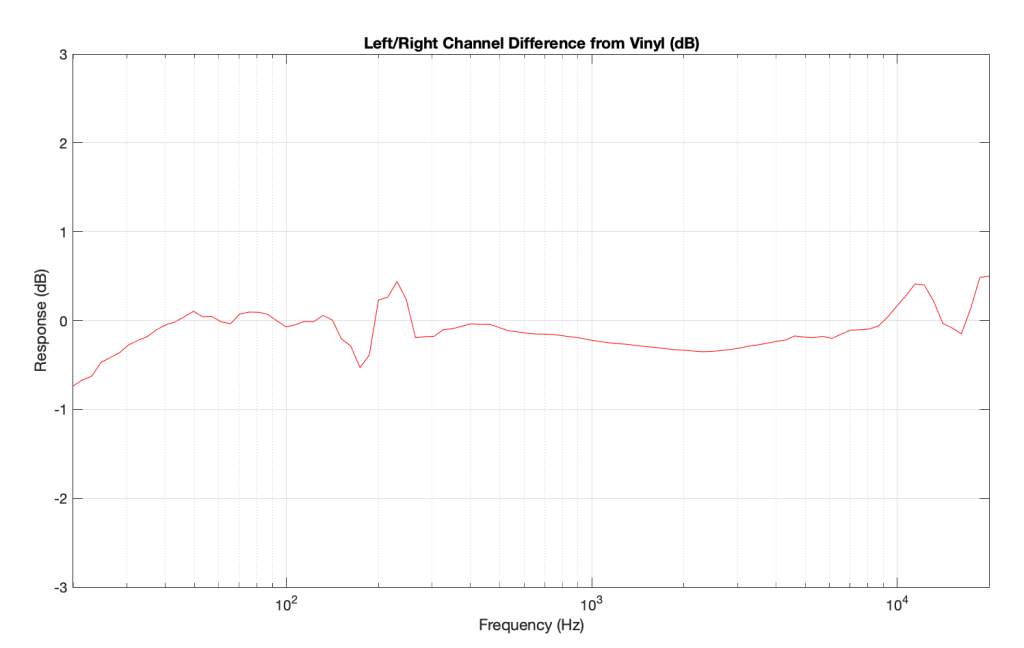
So, we used a stylus brush to clean off the fluff and ran the measurement again. The result immediately afterwards looked like this:
which is more like it! A left-right channel difference of something like ± 0.5 dB is perfectly acceptable.
The moral of the story: keep your pickup clean. But do it carefully! That cantilever is not difficult to snap.
There are many cases where the number of input channels in the audio signal does not match the number of loudspeakers in your configuration. For example, you may have two loudspeakers, but the input signal is from a multichannel source such as a 7.1-channel stream or a 7.1.4-channel Blu-ray. In this case, the audio must be ‘downmixed’ to your two loudspeakers if you are to hear all components of the audio signal. Conversely, you may have a full surround sound system with 7 main loudspeakers and a subwoofer (a 7.1-channel system) and you would like to re-distribute the two channels from a CD to all of your loudspeakers. In this example, the signal must be ‘upmixed’ to all loudspeakers.
Bang & Olufsen’s True Image is a processor that accomplishes both of these tasks dynamically, downmixing or upmixing any incoming signal so that all components and aspects of the original recording are played using all of your loudspeakers.
Of course, using the True Image processor means that signals in the original recording are re-distributed. For example, in an upmixing situation, portions in the original Left Front signal from the source will be sent to a number of loudspeakers in your system instead of just one left front loudspeaker. If you wish to have a direct connection between input and output channels, then the Processing should be set to ‘Direct’, thus disabling the True Image processing.
Note that, in Direct mode, there may be instances where some input or output channels will not be audible. For example, if you have two loudspeakers but a multichannel input, only two of the input channels will be audible. These channels are dependent on the speaker roles selected for the two loudspeakers. (For example, if your loudspeakers’ roles are Left Front and Right Front, then only the Left Front and Right Front channels from the multichannel source will be heard.)
Similarly, in Direct mode, if you have a multichannel configuration but a two-channel stereo input, then only the loudspeakers assigned to have the Left Front and Right Front speaker roles will produce the sound; all other loudspeakers will be silent.
If True Image is selected and if the number of input channels and their channel assignments matches the speaker roles, and if all Spatial Control sliders are set to the middle position, then the True Image processing is bypassed. For example, if you have a 5.1 loudspeaker system with 5 main loudspeakers (Left Front, Right Front, Centre Front, Left Surround, and Right Surround) and a subwoofer, and the Spatial Control sliders are in the middle positions, then a 5.1 audio signal (from a DVD, for example) will pass through unaffected.
However, if the input is changed to a 2.0 source (i.e. a CD or an Internet radio stream) then the True Image processor will upmix the signal to the 5.1 outputs.
In the case where you wish to have the benefits of downmixing without the spatial expansion provided by upmixing, you can choose to use the Downmix setting in this menu. For example, if you have a 5.1-channel loudspeaker configuration and you wish to downmix 6.1- and 7.1-channel sources (thus ensuring that you are able to hear all input channels) but that two-channel stereo sources are played through only two loudspeakers, then this option should be selected. Note that, in Downmix mode, there are two exceptions where upmixing may be applied to the signal. The first of these is when you have a 2.0-channel loudspeaker configuration and a 1-channel monophonic input. In this case, the centre front signal will be distributed to the Left Front and Right Front loudspeakers. The second case is when you have a 6.1 input and a 7.1 loudspeaker configuration. In this case, the Centre Back signal will be distributed to the Left Back and Right Back loudspeakers.
The Beosound Theatre includes four advanced controls (Surround, Height, Stage Width and Envelopment, described below) that can be used to customise the spatial attributes of the output when the True Image processor is enabled.
Surround
The Surround setting allows you to determine the relative levels of the sound stage (in the front) and the surround information from the True Image processor.
Changes in the Surround setting only have an effect on the signal when the Processing is set to True Image.
Height
This setting determines the level of the signals sent to all loudspeakers in your configuration with a ‘height’ Speaker Role. It will have no effect on other loudspeakers in your system.
If the setting is set to minimum, then no signal will be sent to the ‘height’ loudspeakers.
Changes in the Height setting only have an effect on the signal when the Processing is set to True Image.
Stage Width
The Stage Width setting can be used to determine the width of the front images in the sound stage. At a minimum setting, the images will collapse to the centre of the frontal image. At a maximum setting, images will be pushed to the sides of the front sound stage. This allows you to control the perceived width of the band or music ensemble without affecting the information in the surround and back loudspeakers.
If you have three front loudspeakers (Left Front, Right Front and Centre Front), the setting of the Stage Width can be customised according to your typical listening position. If you normally sit in the ‘sweet spot’, at roughly the same distance from all three loudspeakers, then you should increase the Stage Width setting somewhat, since it is unnecessary to use the centre front loudspeaker to help to pull phantom images towards the centre of the sound stage. The further to either side of the sweet spot that you are seated, the more reducing the Stage Width value will improve the centre image location.
Changes in the Stage Width setting only have an effect on the signal when the Processing is set to True Image.
Envelopment
The Envelopment setting allows you to set the desired amount of perceived width or spaciousness from your surround and back loudspeakers. At its minimum setting, the surround information will appear to collapse to a centre back phantom location. At its maximum setting, the surround information will appear to be very wide.
Changes in this setting have no effect on the front loudspeaker channels and only have an effect on the signal when the Processing is set to True Image.
One last point…
One really important thing to know about the True Image processor is that, if the input signal’s configuration matches the output, AND the 4 sliders described above are in the middle positions, then True Image does nothing. In other words, in this specific case, it’s the same as ‘Direct’ mode.
However, if there is a mis-match between the input and the output channel configuration (for example, 2.0 in and 5.1 out, or 7.1.4 in and 5.1.2 out) then True Image will do something: either upmixing or downmixing. Also, if the input configuration matches the output configuration (e.g. 5.x in and 5.x out) but you’ve adjusted any of the sliders, then True Image will also do something…
In 2012, Dolby introduced its Dolby Atmos surround sound technology in movie theatres with the release of the Pixar movie, ‘Brave’, and support for the system was first demonstrated on equipment for home theatres in 2014. However, in spite of the fact that it has been 10 years since its introduction, it still helps to offer an introductory explanation to what, exactly, Dolby Atmos is. For more in-depth explanations, https://www.dolby.com/technologies/dolby-atmos is a good place to start and https://www.dolby.com/about/support/guide/speaker-setup-guides has a wide range of options for loudspeaker configuration recommendations.
From the perspective of audio / video systems for the home, Dolby Atmos can most easily be thought of as a collection of different things:
a set of recommendations for loudspeaker configuration that can include loudspeakers located above the listening position
a method of supplying audio signals to those loudspeakers that not only use audio channels that are intended to be played by a single loudspeaker (e.g. Left Front or Right Surround), but also audio objects whose intended spatial positions are set by the mixing engineer, but whose actual spatial position is ‘rendered’ based on the actual loudspeaker configuration in the customer’s listening room.
a method of simulating the spatial positions of ‘virtual’ loudspeakers
the option to use loudspeakers that are intentionally directed away from the listening position, potentially increasing the spatial effects in the mix. These are typically called ‘up-firing’ and ‘side-firing’ loudspeakers.
In addition to this, Dolby has other technologies that have been enhanced to be used in conjunction with Dolby Atmos-encoded signals. Arguably, the most significant of these is an upmixing / downmixing algorithm that can adapt the input signal’s configuration to the output channels.
Note that many online sites state that Dolby’s upmixing / downmixing processor is part of the Dolby Atmos system. This is incorrect. It’s a separate processor.
1. Loudspeaker configurations
Dolby’s Atmos recommendations allow for a large number of different options when choosing the locations of the loudspeakers in your listening room. These range from a simple 2.0.0, traditional two-channel stereo loudspeaker configuration up to a 24.1.10 large-scale loudspeaker array for movie theatres. The figures below show a small sampling of the most common options. (see https://www.dolby.com/about/support/guide/speaker-setup-guides/ for many more possibilities and recommendations.)
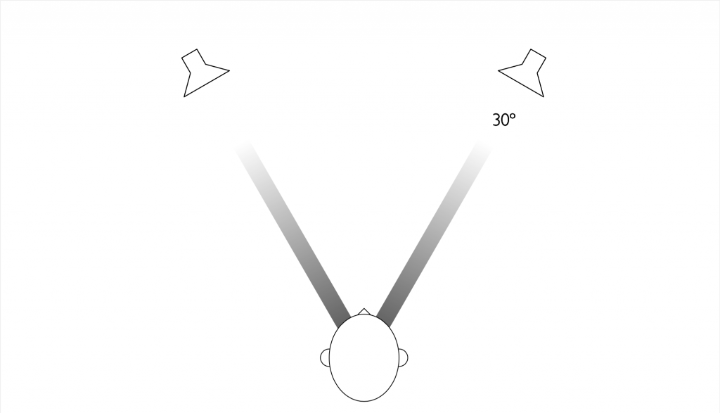
Standard loudspeaker configuration for two-channel stereo (Lf / Rf)
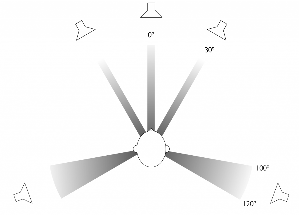
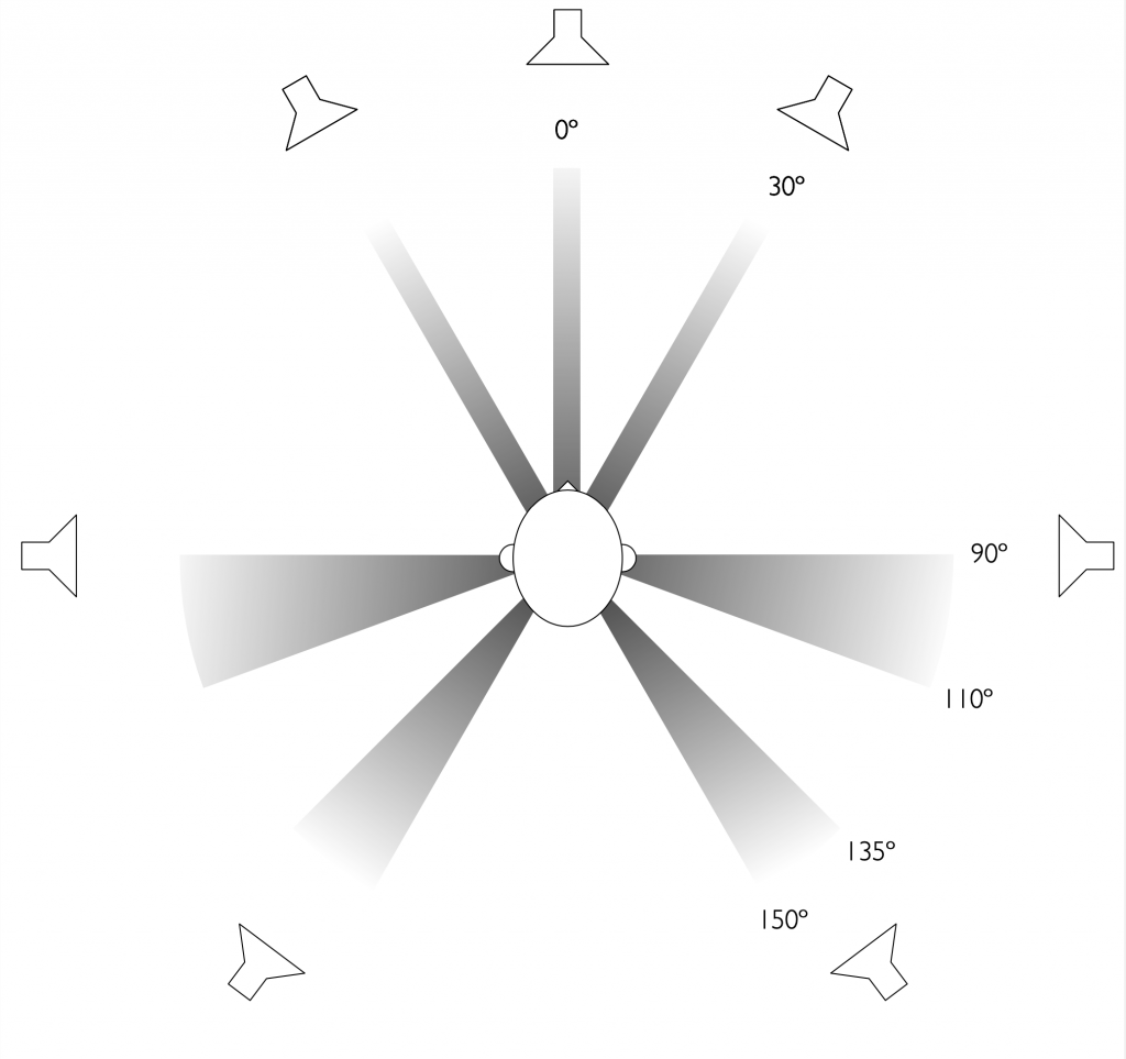
Standard loudspeaker configuration for 5.x multichannel audio. The actual angles of the surround loudspeakers at 110 degrees shows the reference placement used at Bang & Olufsen for testing and tuning. Note that the placement of the subwoofer is better determined by your listening room’s acoustics, but it is advisable to begin with a location near the centre front loudspeaker.
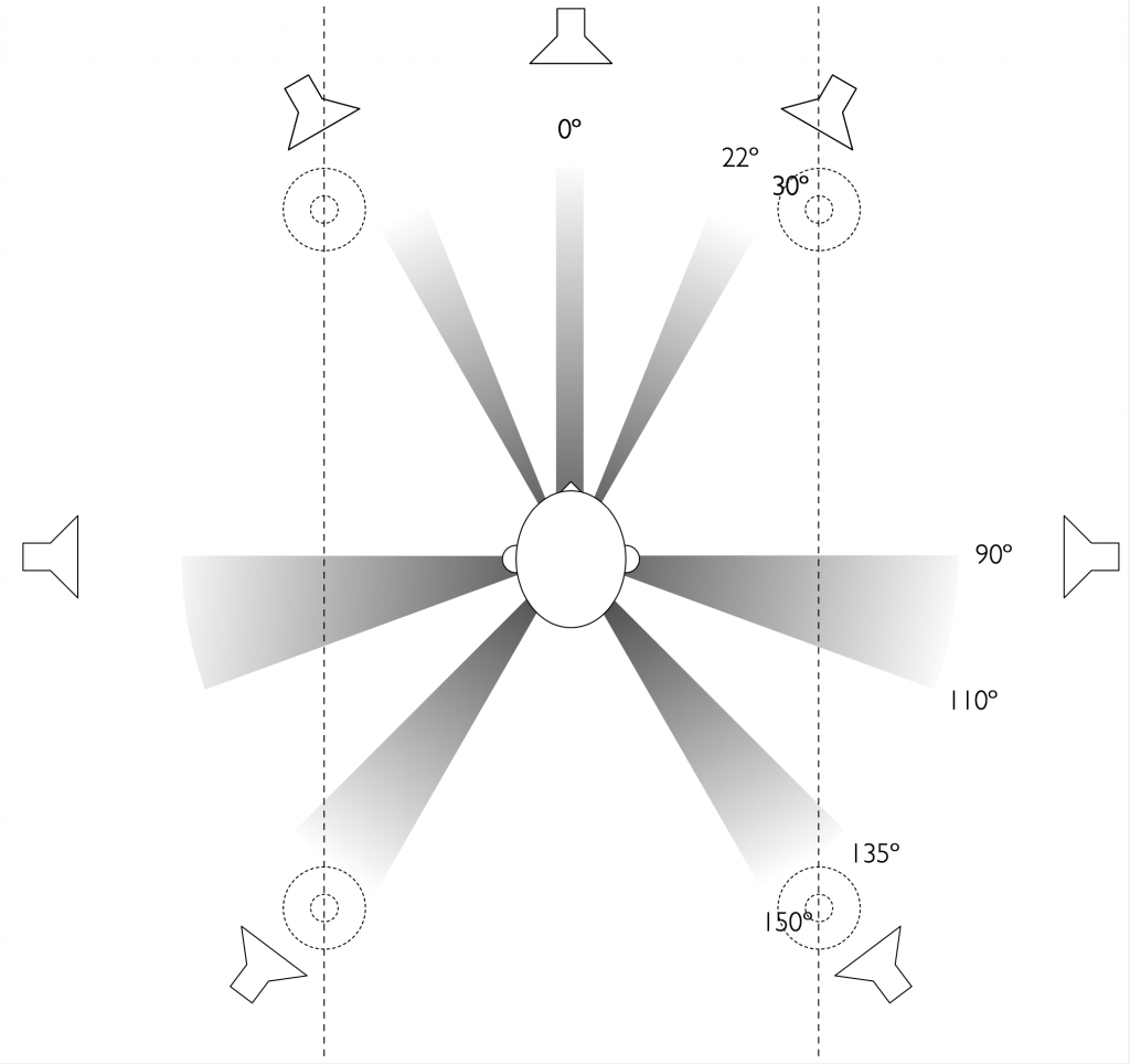
Recommended loudspeaker configuration for most 7.x channel audio signals. The actual angles of the loudspeakers shows the reference placement used at Bang & Olufsen for testing and tuning.Loudspeaker positions associated with the speaker roles available in the Beosound Theatre, showing a full 7.x.4 configuration.
Loudspeaker positions associated with the speaker roles available in the Beosound Theatre, showing a full 7.x.4 configuration.
2. Channels and Objects
Typically, when you listen to audio, regardless of whether it’s monophonic or a stereo (remember that ‘stereo’ merely implies ‘more than one channel’) signal, you are reproducing some number of audio channels that were mixed in a studio. For example, a recording engineer placed a large number of microphones around a symphony orchestra or a jazz ensemble, and then decided on the mix (or relative balance) of those signals that should be sent to a loudspeakers in the left front and right front positions. They did this by listening to the mix through loudspeakers in a standard configuration with the intention that you place your loudspeakers similarly and sit in the correct location.
Consequently, each loudspeaker’s input can be thought of as receiving a ‘pre-packaged’ audio channel of information.
However, in the early 2000s, a new system for delivering audio to listeners was introduced with the advent of powerful gaming consoles. In these systems, it was impossible for the recording engineer to know where a sound should be coming from at any given moment in a game with moving players. So, instead of pre-mixing sound effects (like footsteps, for example) in a fixed position, a monophonic recording of the effect (the footsteps) was stored in the game’s software, and then the spatial position could be set at the moment of playback. So, if the footsteps should appear on the player’s left, then the game console would play them on the left. If the player then turned, the footsteps could be moved to appear in the centre or on the right. In this way different sound objects could be ‘rendered’ instead of merely being reproduced. Of course, the output of these systems was still either loudspeakers or headphones; so the rendered sound objects were mixed with the audio channels (e.g. background music) before being sent to the outputs.
The advantage of a channel-based system is that there is (at least theoretically) a 1:1 match between what the recording or mastering engineer heard in the studio, and what you are able to hear at home. The advantage of an object-based system is that it can not only adapt to the listener’s spatial changes (e.g. the location and rotation of a player inside a game environment) but also to changes in loudspeaker configurations. Change the loudspeakers, and you merely tell the system to render the output differently.
Dolby’s Atmos system merges these two strategies, delivering audio content using both channel-based and object-based streams. By delivering audio channels that match older systems, it becomes possible to have a mix on a newly-released movie that is compatible with older playback systems. However, newer Dolby Atmos-compatible systems can render the object-based content as well, optimising the output for the particular configuration of the loudspeakers.
3. Virtual Loudspeakers
Dolby’s Atmos processing includes the option to simulate loudspeakers in ‘virtual’ locations using ‘real’ loudspeakers placed in known locations. Beosound Theatre uses this Dolby Atmos processing to generate the signals used to create four virtual outputs. (This is discussed in detail in another posting.)
4. Up-firing and Side-firing Loudspeakers
A Dolby Atmos-compatible soundbar or loudspeaker can also include output beams that are aimed away from instead of towards the listening position; either to the sides or above the loudspeakers.
These are commonly known as ‘up-firing’ and ‘side-firing’ loudspeakers. Although Beosound Theatre gives you the option of using a similar concept, it is not merely implemented with a single loudspeaker driver, but with a version of the Beam Width and Beam Direction control used in other high-end Bang & Olufsen loudspeakers. This means that, when using the up-firing and side-firing outputs, more than a single loudspeaker driver is being used to produce the sound. This helps to reduce the beam width, reducing the level of the direct sound at the listening position, which, in turn can help to enhance the spatial effects that can be encoded in a Dolby Atmos mix.
Upmixing and Downmixing
There are cases where an incoming audio signal was intended to be played by a different number of loudspeakers than are available in the playback system. In some cases, the playback uses fewer loudspeakers (e.g. when listening to a two-channel stereo recording on the single loudspeaker on a mobile phone). In other cases, the playback system has more loudspeakers (e.g. when listening to a monophonic news broadcast on a 5.1 surround sound system). When the number of input channels is larger than the number of outputs (typically loudspeakers), the signals have to be downmixed so that you are at least able to hear all the content, albeit at the price of spatially-distorted reproduction. (For example, instruments will appear to be located in incorrect locations, and the spaciousness of a room’s reverberation may be lost.) When the number of output channels (loudspeakers) is larger than the number of input channels, then the system may be used to upmix the signal.
The Dolby processor in a standard playback device has the capability of performing both of these tasks: either upmixing or downmixing when required (according to both the preferences of the listener). One particular feature included in this processing is the option for a mixing engineer to ‘tell’ the playback system exactly how to behave when doing this. For example, when downmixing a 5.1-channel movie to a two-channel output, it may be desirable to increase the level of the centre channel to increase the level of the dialogue to help make it more intelligible. Dolby’s encoding system gives the mixing engineer this option using ‘metadata’; a set of instructions defining the playback system’s behaviour so that it behaves as intended by the artist (the mixing engineer). Consequently, the Beosound Theatre gives you the option of choosing the Downmix mode, where this processing is done exclusively in the Dolby processor.
However, there are also cases where you may also wish to upmix the signal to more loudspeakers than there are input channels from the source material. For these situations, Bang & Olufsen has developed its own up-/down-mixing processor called True Image, which I’ll discuss in more detail in another posting.
Once upon a time, in the incorrectly-named ‘Good Old Days’, audio systems were relatively simple things. There was a single channel of audio picked up by a gramophone needle or transmitted to a radio, and that single channel was reproduced by a single loudspeaker. Then one day, in the 1930s, a man named Alan Blumlein was annoyed by the fact that, when he was watching a film at the cinema and a character moved to one side of the screen, the voice still sounded like it was coming from the centre (because that’s where the loudspeaker was placed). So, he invented a method of simultaneously reproducing more than one channel of audio to give the illusion of spatial changes. (See Patent GB394325A:Improvements in and relating to sound-transmission, sound-recording and sound-reproducing systems’) Eventually, that system was called stereophonic audio.
The word stereo’ first appeared in English usage in the late 1700s, borrowed directly from the French word ‘stéréotype’: a combination of the Greek word στερεó (roughly pronounced ‘stereo’) meaning ‘solid’ and the Latin ‘typus’ meaning ‘form’. ‘Stereotype’ originally meant a letter (the ‘type’) printed (e.g. on paper) using a solid plate (the ‘stereo’). In the mid-1800s, the word was used in ‘stereoscope’ for devices that gave a viewer a three-dimensional visual representation using two photographs. So, by the time Blumlein patented spatial improvements in audio recording and reproduction in the 1930s, the word had already been in used to mean something akin to ‘a three-dimensional representation of something’ for over 80 years.
Over the past 90 years, people have come to mis-understand that ‘stereo’ audio implies only two channels, but this is incorrect, since Blumlein’s patent was also for three loudspeakers, placed on the left, centre, and right of the cinema screen. In fact, a ‘stereo’ system simply means that it uses more than one audio channel to give the impression of sound sources with different locations in space. So it can easily be said that all of the other names that have been used for multichannel audio formats (like ‘quadraphonic’, ‘surround sound’, ‘multichannel audio’, and ‘spatial audio’, just to name a few obvious examples) since 1933 are merely new names for ‘stereo’ (a technique that we call ‘rebranding’ today).
At any rate, most people were introduced to `stereophonic’ audio either through a two-channel LP, cassette tape, CD, or a stereo FM radio receiver. Over the years, systems with more and more audio channels have been developed; some with more commercial success than others. The table below contains a short list of examples.
Some of the information in that list may be surprising, such as the existence of a 7-channel audio system in the 1950s, for example. Another interesting thing to note is the number of multichannel formats that were not `merely’ an accompaniment to a film or video format.
One problem that is highlighted in that list is the confusion that arises with the names of the formats. One good example is ‘Dolby Digital’, which was introduced as a name not only for a surround sound format with 5.1 audio channels, but also the audio encoding method that was required to deliver those channels on optical film. So, by saying ‘Dolby Digital’ in the mid-1990s, it was possible that you meant one (or both) of two different things. Similarly, although SACD and DVD-Audio were formats that were capable of supporting up to 6 channels of audio, there was no requirement and therefore no guarantee that the content be multichannel or that the LFE channel actually contain low-frequency content. This grouping of features under one name still causes confusion when discussing the specifics of a given system, as we’ll discuss below in the section on Dolby Atmos.
Format
Introduced
Channels
Note
Edison phonograph cylinders
1896
1
Berliner gramophone record
1897
1
Wire recorder
1898
1
Optical (on film)
ca. 1920
1
Magnetic Tape
1928
2
Fantasound
1940
3 / 54
3 channels through 54 loudspeakers
Cinerama
1950s
7.1
Actually 7 channels
Stereophonic LP
1957
2
Compact Cassette
1963
2
Q-8 magnetic tape cartridge
1970
4
CD-4 Quad LP
1971
4
SQ (Stereo Quadraphonic) LP
1971
4
IMAX
1971
5.1
Dolby Stereo
1975
4
aka Dolby Surround
Compact Disc
1983
2
DAT
1987
2
Mini-disc
1992
2
Digital Compact Cassette
1992
2
Dolby Digital
1992
5.1
DTS Coherent Acoustics
1993
5.1
Sony SDDS
1999
7.1
SACD
1999
5.1
Actually 6 full-band channels
Dolby EX
1999
6.1
Tom Holman / TMH Labs
1999
10.2
DVD-Audio
2000
5.1
Actually 6 full-band channels
DTS ES
2000
6.1
NHK Ultra-high definition TV
2005
22.2
Auro 3D
2005
9.1 to 26.1
Dolby Atmos
2012
up to 24.1.10
Looking at the column listing the number of audio channels in the different formats, you may have three questions:
Why does it say only 4 channels for Dolby Stereo? I saw Star Wars in the cinema, and I remember a LOT more loudspeakers on the walls.
What does the `.1′ mean? How can you have one-tenth of an audio channel?
Some of the channel listings have one or two numbers and some have three, which I’ve never seen before. What do the different numbers represent?
Input Channels and Speaker Roles
A ‘perfect’ two-channel stereo system is built around two matched loudspeakers, one on the left and the other on the right, each playing its own dedicated audio channel. However, when better sound systems were developed for movie theatres, the engineers (starting with Blumlein) knew that it was necessary to have more than two loudspeakers because not everyone is sitting in the middle of the theatre. Consequently, a centre loudspeaker was necessary to give off-centre listeners the impression of speech originating in the middle of the screen. In addition, loudspeakers on the side and rear walls helped to give the impression of envelopment for effects such as rain or crowd noises.
It is recommended but certainly not required, that a given Speaker Role should only be directed to one loudspeaker. In a commercial cinema, for example, a single surround channel is most often produced by many loudspeakers arranged on the side and rear walls. This can also be done in larger home installations where appropriate.
Similarly, in cases where the Beosound Theatre is accompanied by two larger front loudspeakers, it may be preferable to use the three front-firing outputs to all produce the Centre Front channel (instead of using the centre output only).
x.1 ?
The engineers also realised that it was not necessary that all the loudspeakers be big, and therefore requiring powerful amplifiers. This is because larger loudspeakers are only required for high-level content at low frequencies, and we humans are terrible at locating low-frequency sources when we are indoors. This meant that effects such as explosions and thunder that were loud, but limited to the low-frequency bands could be handled by a single large unit instead; one that handled all the content below the lowest frequencies capable of being produced by the other loudspeakers’ woofers. So, the systems were designed to rely on a powerful sub-woofer that driven by a special, dedicated Low Frequency Effects (or LFE) audio channel whose signals were limited up to about 120 Hz. However, as is discussed in the section on Bass Management, it should not be assumed that the LFE input channel is only sent to a subwoofer; nor that the only signal produced by the subwoofer is the LFE channel. This is one of the reasons it’s important to keep in mind that the LFE input channel and the subwoofer output channel are separate concepts.
Since the LFE channel only contains low frequency content, it has only a small fraction of the bandwidth of the main channels. (‘Bandwidth’ is the total frequency width of the signal. In the case of the LFE channel it is up to about 120 Hz. (In fact, different formats have different bandwidths for the LFE channel, but 120 Hz is a good guess.) In the case of a main channel, it is up to about 20,000 Hz; however these values are not only fuzzy but dependent on the specifications of distribution format, for example.) Although that fraction is approximately 120/20000, we generously round it up to 1/10 and therefore say that, relative to a main audio channel like the Left Front, the LFE signal is only 0.1 of a channel. Consequently, you’ll see audio formats with something like ‘5.1 channels’ meaning `5 main channels and an LFE channel’. (This is similar to the way rental apartments are listed in Montr\’eal, where it’s common to see a description such as a 3 1/2; meaning that it has a living room, kitchen, bedroom, and a bathroom (which is obviously half of a room).)
LFE ≠ Subwoofer
Many persons jump to the conclusion that an audio input with an LFE channel (for example, a 5.1 or a 7.1.4 signal) means that there is a ‘subwoofer’ channel; or that a loudspeaker configuration with 5 main loudspeakers and a subwoofer is a 5.1 configuration. It’s easy to make this error because those are good descriptions of the way many systems have worked in the past.
However, systems that use bass management break this direct connection between the LFE input and the subwoofer output. For example, if you have two large loudspeakers such as Beolab 50s or Beolab 90s for your Lf / Rf pair, it may not be necessary to add a subwoofer to play signals with an LFE channel. In fact, in these extreme cases, adding a subwoofer could result in downgrading the system. Similarly, it’s possible to play 2.0-channel signal through a system with two smaller loudspeakers and a single subwoofer.
Therefore, it’s important to remember that the ‘x.1’ classification and the discussion of an ‘LFE’ channel are descriptions of the input signal. The output may or may not have one or more subwoofers; and these two things are essentially made independent of each other using a bass management system.
x.y.4 ?
If you look at the table above, you’ll see that some formats have very large numbers of channels, however, these numbers can be easily mis-interpreted. For example, in both the ‘10.2’ and ‘22.2’ systems, some of the audio channels are intended to be played through loudspeakers above the listeners, but there’s no way to know this simply by looking at the number of channels. This is why we currently use a new-and-improved method of listing audio channels with three numbers instead of two.
The first number tells you how many ‘main’ audio channels there are. In an optimal configuration, these should be reproduced using loudspeakers at the listeners’ ear heights.
The second number tells you how many LFE channels there are.
The third number tells you how many audio channels are intended to be reproduced by loudspeakers located above the listeners.
For example, you’ll notice looking at the table below, that a 7.1.4 channel system contains seven main channels around the listeners, one LFE channel, and four height channels.
Speaker Role
2.0
5.1
7.1
7.1.4
Left Front
x
x
x
x
Right Front
x
x
x
x
Centre Front
x
x
x
LFE
x
x
x
Left Surround
x
x
x
Right Surround
x
x
x
Left Back
x
x
Right Back
x
x
Left Front Height
x
Right Front Height
x
Left Surround Height
x
Right Surround Height
x
It is worth noting here that the logic behind the Bang & Olufsen naming system is either to avoid having duplicate letters for different role assignments, or to reserve options for future formats. For example, ‘Back’ is used instead of ‘Rear’ to prevent confusion with ‘Right, and ‘Height’ is used instead of ‘Top’ because another, higher layer of loudspeakers may be used in future formats. (The ‘Ceiling’ loudspeaker channel used in multichannel recordings from Telarc is an example of this.)
Beosound Theatre has a total of 11 possible outputs, seven of which are “real” or “internal” outputs and four of which are “virtual” loudspeakers. As with all current Beovision televisions, any input channel can be directed to any output by setting the Speaker Roles in the menus.
Internal outputs
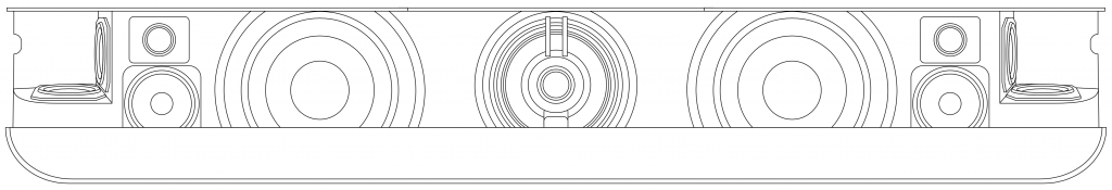
On first glance of the line drawing above it is easy to jump to the conclusion that the seven real outputs are easy to find, however this would be incorrect. The Beosound Theatre has 12 loudspeaker drivers that are all used in some combination of level and phase at different frequencies to all contribute to the total result of each of the seven output channels.
So, for example, if you are playing a sound from the Left front-firing output, you will find that you do not only get sound from the left tweeter, midrange, and woofer drivers as you might in a normal soundbar. There will also be some contribution from other drivers at different frequencies to help control the spatial behaviour of the output signal. This Beam Width control is similar to the system that was first introduced by Bang & Olufsen in the Beolab 90. However, unlike the Beolab 90, the Width of the various beams cannot be changed in the Beosound Theatre.
The seven internal loudspeaker outputs are
Front-firing: Left, Centre, and Right
Side-firing: Left and Right
Up-firing: Left and Right
Looking online, you may find graphic explanations of side-firing and up-firing drivers in other loudspeakers. Often, these are shown as directing sound towards a reflecting wall or ceiling, with the implication that the listener therefore hears the sound in the location of the reflection instead. Although this is a convenient explanation, it does not necessarily match real-life experience due to the specific configuration of your system and the acoustical properties of the listening room.
The truth is both better and worse than this reductionist view. The bad news is that the illusion of a sound coming from a reflective wall instead of the loudspeaker can occur, but only in specific, optimised circumstances. The good news is that a reflecting surface is not strictly necessary; therefore (for example) side-firing drivers can enhance the perceived width of the loudspeaker, even without reflecting walls nearby.
However, it can be generally said that the overall benefit of side- and up-firing loudspeaker drivers is an enhanced impression of the overall width and height of the sound stage, even for listeners that are not seated in the so-called “sweet spot” (see Footnote 1) when there is appropriate content mixed for those output channels.
Virtual outputs
Devices such as the “stereoscope” for representing photographs (and films) in three-dimensions have been around since the 1850s. These work by presenting two different photographs with slightly different perspectives two the two eyes. If the differences in the photographs are the same as the differences your eyes would have seen had you “been there”, then your brain interprets into a 3D image.
A similar trick can be done with sound sources. If two different sounds that exactly match the signals that you would have heard had you “been there” are presented at your two ears (using a binaural recording) , then your brain will interpret the signals and give you the auditory impression of a sound source in some position in space. The easiest way to do this is to ensure that the signals arriving at your ears are completely independent using headphones.
The problem with attempting this with loudspeaker reproduction is that there is “crosstalk” or “bleeding of the signals to the opposite ears”. For example, the sound from a correctly-positioned Left Front loudspeaker can be heard by your left ear and your right ear (slightly later, and with a different response). This interference destroys the spatial illusion that is encoded in the two audio channels of a binaural recording.
However, it might be possible to overcome this issue with some careful processing and assumptions. For example, if the exact locations of the left and right loudspeakers and your left and right ears are known by the system, then it’s (hypothetically) possible to produce a signal from the right loudspeaker that cancels the sound of the left loudspeaker in the right ear, and therefore you only hear the left channel in the left ear. (see Footnote 2)
Using this “crosstalk cancellation” processing, it becomes (hypothetically) possible to make a pair of loudspeakers behave more like a pair of headphones, with only the left channel in the left ear and the right in the right. Therefore, if this system is combined with the binaural recording / reproduction system, then it becomes (hypothetically) possible to give a listener the impression of a sound source placed at any location in space, regardless of the actual location of the loudspeakers.
Theory vs. Reality
It’s been said that the difference between theory and practice is that, in theory, there is no difference between theory and practice, whereas in practice, there is. This is certainly true both of binaural recordings (or processing) and crosstalk cancellation.
In the case of binaural processing, in order to produce a convincing simulation of a sound source in a position around the listener, the simulation of the acoustical characteristics of a particular listener’s head, torso, and (most importantly) pinnæ (a.k.a. “ears”) must be both accurate and precise. (see Footnote 3)
Similarly, a crosstalk cancellation system must also have accurate and precise “knowledge” of the listener’s physical characteristics in order to cancel the signals correctly; but this information also crucially includes the exact locations of the loudspeakers and the listener (we’ll conveniently pretend that the room you’re sitting in does not exist).
In the end, this means that a system with adequate processing power can use two loudspeakers to simulate a “virtual” loudspeaker in another location. However, the details of that spatial effect will be slightly different from person to person (because we’re all shaped differently). Also, more importantly, the effect will only be experienced by a listener who is positioned correctly in front of the loudspeakers. Slight movements (especially from side-to-side, which destroys the symmetrical time-of-arrival matching of the two incoming signals) will cause the illusion to collapse.
Beosound Theatre gives you the option to choose Virtual Loudspeakers that appear to be located in four different positions: Left and Right Wide, and Left and Right Elevated. These signals are actually produced using the Left and Right front-firing outputs of the device using this combination of binaural processing and crosstalk cancellation in the Dolby Atmos processing system. If you are a single listener in the correct position (with the Speaker Distances and Speaker Levels adjusted correctly) then the Virtual outputs come very close to producing the illusion of correctly-located Surround and Front Height loudspeakers.
However, in cases where there is more than one listener, or where a single listener may be incorrectly located, it may be preferable to use the “side-firing” and “up-firing” outputs instead.
Wrapping up
As I mentioned at the start, Beosound Theatre on its own has 11 outputs:
Front-firing: Left, Centre, and Right
Side-firing: Left and Right
Up-firing: Left and Right
Virtual Wide: Left and Right
Virtual Elevated: Left and Right
In addition to these, there are 8 wired Power Link outputs and 8 Wireless Power Link outputs for connection to external loudspeakers, resulting in a total of 27 possible output paths. And, as is the case with all Beovision televisions since Beoplay V1, any input channel (or output channel from the True Image processor) can be directed to any output, giving you an enormous range of flexibility in configuring your system to your use cases and preferences.
1. In the case of many audio playback systems, the “sweet spot” is directly in front of the loudspeaker pair or at the centre of the surround configuration. In the case of a Bang & Olufsen system, the “sweet spot” is defined by the user with the help of the Speaker Distance and Speaker Level adjustments.
2. Of course, the cancelling signal of the right loudspeaker also bleeds to the left ear, so the left loudspeaker has to be used to cancel the cancellation signal of the right loudspeaker in the left ear, and so on…
3. For the same reason that someone else should not try to wear my glasses.
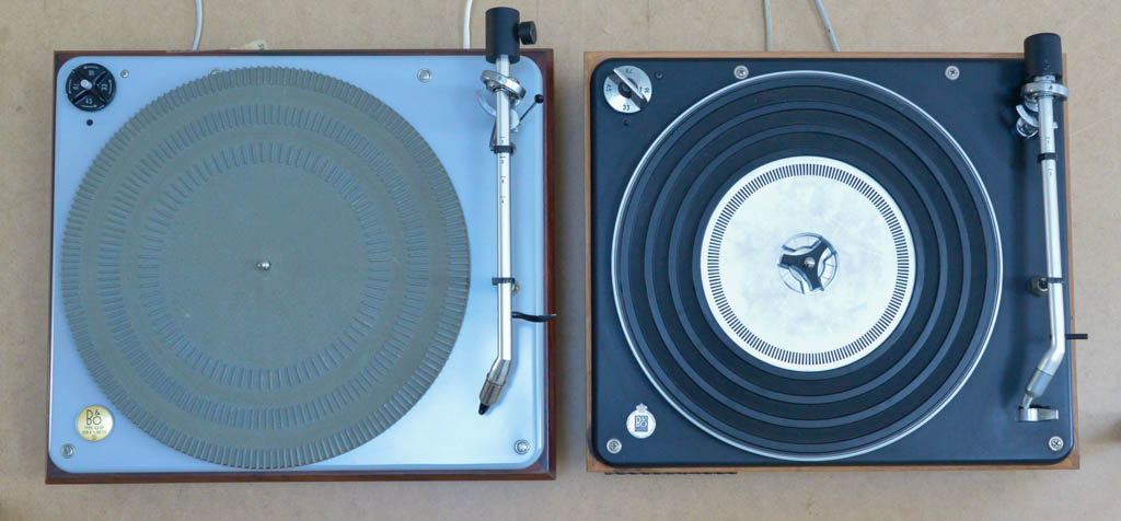
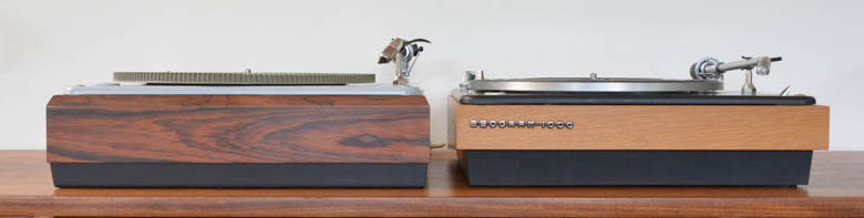
On the left: a “Stereopladespiller” (Stereo Gramophone) Type 42 VF. On the right, a Beogram 1000 V Type 5203 Series 33, modified with a built-in RIAA preamp (making it a Beogram 1000 VF)
Some history today – without much tech-talk. I just finished restoring my 42VF and I thought I’d spend an hour or two taking some photos next to my BG1000.
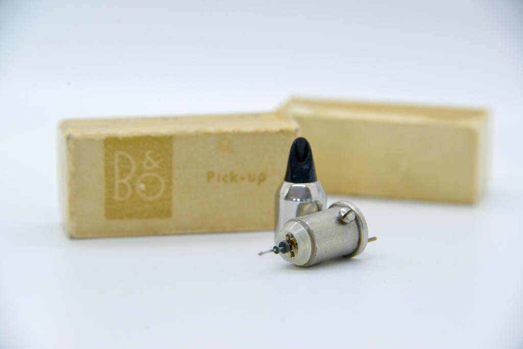
According to the beoworld.org website, the Stereopladespiller was in production from 1960 to 1976. Although Bang & Olufsen made many gramophones before 1960, they were all monophonic, for 1-channel audio. This one was originally made to support the 2-channel “SP1 / SP2” pickup developed by Erik Rørbæk Madsen after having heard 2-channel stereo on a visit to the USA in the mid-1950s (and returned to Denmark with a test record).
Sidebar: The “V” means that the players are powered from the AC mains voltage (220 V AC, 50 Hz here in Denmark). The “F” stands for “Forforstærker” or “Preamplifier”, meaning that it has a built-in RIAA preamp with a line-level output.
Internally, the SP1 and SP2 are identical. The only difference is the mounting bracket to accommodate the B&O “ST-” series tonearms and standard tonearms.
Name, Pivot – Platter Centre, Pivot – Stylus, Pickup
ST/M,190 mm, 205 mm, SP2
ST/L, 209.5 mm, 223.5 mm, SP2
ST/P, 310 mm, 320 mm, SP2
ST/A, 209.5 mm, 223.5 mm, SP1
[/table]
(I’ll do another, more detailed posting about the tonearms at a later date…)
Again, according to the beoworld.org website, the Beogram 1000 was in production from 1965 to 1973. (The overlap and the later EoP date of the former makes me a little suspicious. If I get better information, I’ll update this posting.)
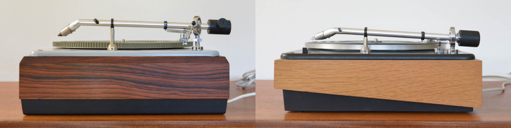
The tonearm seen here on the Stereopladespiller is the ST/L model with a Type PL tonearm lifter.
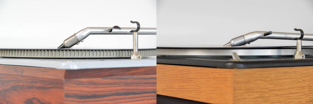
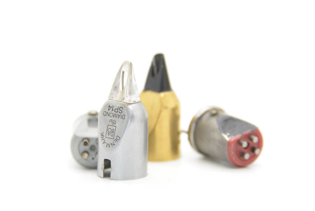
Looking not-very-carefully at the photos below, you can see that the two tonearms have a significant difference – the angle of the pickup relative to the surface of the vinyl. The ST/L has a 25º angle whereas the tonearm on the Beogram 1000 has a 15º angle. This means that the two pickups are mutually incompatible. The pickup shown on the Beogram 1000 is an SP14.
This, in turn, means that the vertical pivot points for the two tonearms are different, as can be seen below.
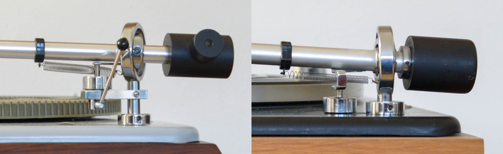
The heights of both tonearms at the pivot are adjustable by moving a collar around the post and fixing its position with a small set screw. A nut under the top plate (inside the turntable) locks it in position.
The position of the counterbalance on the older tonearm can be adjusted with the large setscrew seen in the photo above. The tonearm on the Beogram 1000 gently “locks” into the correct position using a small spring-loaded ball that sets into a hole at the end of the tonearm tube, and so it’s not designed to have the same adjustability.
Both tonearms use a spring attached to a plastic collar with an adjustable position for fine-tuning the tracking force. At the end of this posting, you can see that I’ve measured its accuracy.
The Micro Moving Cross (MMC) principle of the SP1/2 pickup can easily be seen in the photo above (a New-Old-Stock pickup that I stumbled across at a flea market). For more information about the MMC design, see this posting. In later versions of the pickup, such as the SP14, seen below, the stylus and MMC assembly were attached to the external housing instead.
A couple of later SP-series pickups in considerably worse shape. These are also flea-market finds, but neither of them is behaving very well due to bent cantilevers.
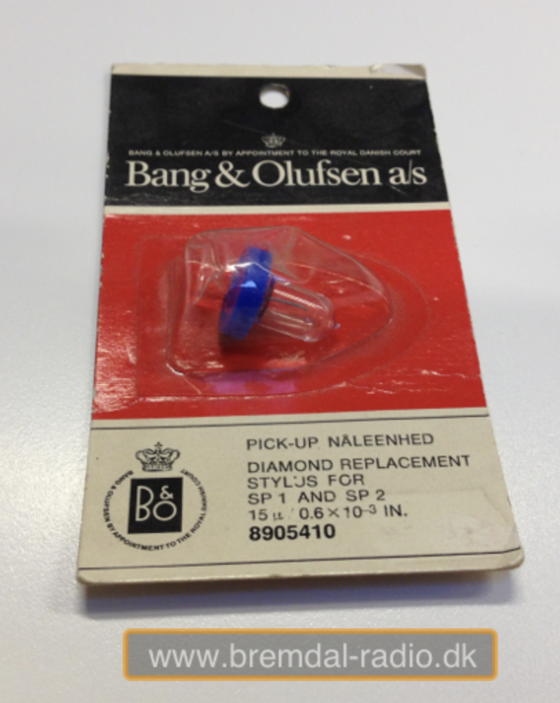
This construction made it easier to replace the stylus, although it was also possible to do so with the SP1-2 using a replacement such as the one shown below.
A replacement stylus for the SP1/2 shown on the bremdal-radio.dk website.
Just to satisfy my own curiosity, I measured the tracking force at the stylus with a number of different adjustments on the collar. The results are shown below.
Tracking force on the Stereopladespiller with the collar aligned to each side of the gradations on the tonearm. Right-click on the photo and open it in a new window or tab to zoom in for more details.Tracking force on the Beogram 1000 with the collar aligned to each side of the gradations on the tonearm. Right-click on the photo and open it in a new window or tab to zoom in for more details.
As you can see there, the accuracy is reasonably good. This is not really surprising, since the tracking force is applied by a spring. So, as long as the spring constant hasn’t changed over the years, which it shouldn’t have unless it got stretched for some reason (say, when I was rebuilding the pivot on the tonearm, for example…) it should behave as it always did.
In a perfect sound system, all loudspeakers are identical, and they are all able to play a full frequency range at any listening level. However, most often, this is not a feasible option, either due to space or cost considerations (or both…). Luckily, it is possible to play some tricks to avoid having to install a large-scale sound system to listen to music or watch movies.
Humans have an amazing ability to localise sound sources. With your eyes closed, you are able to point towards the direction sounds are coming from with an incredible accuracy. However, this ability gets increasingly worse as we go lower in frequency, particularly in closed rooms.
In a sound system, we can use this inability to our advantage. Since you are unable to localise the point of origin of very low frequencies indoors, it should not matter where the loudspeaker that’s producing them is positioned in your listening room. Consequently, many simple systems remove the bass from the “main” loudspeakers and send them to a single large loudspeaker whose role it is to reproduce the bass for the entire system. This loudspeaker is called a “subwoofer”, since it is used to produce frequency bands below those played by the woofers in the main loudspeakers.
The process of removing the bass from the main channels and re-routing them to a subwoofer is called bass management.
It’s important to remember that, although many bass management systems assume the presence of at least one subwoofer, that output should not be confused with an (Low-Frequency Effects) LFE (Low-Frequency Effects) or a “.1” input channel. However, in most cases, the LFE channel from your media (for example, a Blu-ray disc or video streaming device) will be combined with the low-frequency output of the bass management system and the total result routed to the subwoofer. A simple example of this for a 5.1-channel system is shown below in Figure 1.
Figure 1: A simple example of a bass management system for a 5.1 channel system.
Of course, there are many other ways to do this. One simplification that’s usually used is to put a single Low Pass Filter (LPF) on the output of the summing buss after the signals are added together. That way, you only need to have the processing for one LPF instead of 5 or 6. On the other hand, you might not want to apply a LPF to an LFE input, so you may want to add the main channels, apply the LPF, and then add the LFE, for example. Other systems such as Bang & Olufsen televisions use a 2-channel bass management system so that you can have two subwoofers (or two larger main loudspeakers) and still maintain left/right differences in the low frequency content all the way out to the loudspeakers.
However, the one thing that older bass management systems have in common is that they typically route the low frequency content to a subset of the total number of loudspeakers. For example, a single subwoofer, or the two main front loudspeakers in a larger multichannel system.
In Bang & Olufsen televisions starting with the Beoplay V1 and going through to the Beovision Harmony, it is possible to change this behaviour in the setup menus, and to use the “Re-direction Level” to route the low frequency output to any of the loudspeakers in the current Speaker Group. So, for example, you could choose to send the bass to all loudspeakers instead of just one subwoofer.
There are advantages and disadvantages to doing this.
The first advantage is that, by sending the low frequency content to all loudspeakers, they all work together as a single “subwoofer”, and thus you might be able to get more total output from your entire system.
The second advantage is that, since the loudspeakers are (probably) placed in different locations around your listening room, then they can work together to better control the room’s resonances (a.k.a. room modes).
One possible disadvantage is that, if you have different loudspeakers in your system (say, for example, Beolab 3s, which have slave drivers, and Beolab 17s, which use a sealed cabinet design) then your loudspeakers may have different frequency-dependent phase responses. This can mean in some situations that, by sending the same signal to more loudspeakers, you get a lower total acoustic output in the room because the loudspeakers will cancel each other rather than adding together.
Another disadvantage is that different loudspeakers have different maximum output levels. So, although they may all have the same output level at a lower listening level, as you turn the volume up, that balance will change depending on the signal level (which is also dependent on frequency content). For example, if you own Beolab 17s (which are small-ish) and Beolab 50s (which are not) and if you’re listening to a battle scene with lots of explosions, at lower volume levels, the 17s can play as much bass as the 50s, but as you turn up the volume, the 17s reach their maximum limit and start protecting themselves long before the 50s do – so the balance of bass in the room changes.
Beosound Theatre
Beosound Theatre uses a new Bass Management system that is an optimised version of the one described above, with safeguards built-in to address the disadvantages. To start, the two low-frequency output channels from the bass management system are distributed to all loudspeakers in the system that are currently being used.
However, in order to ensure that the loudspeakers don’t cancel each other, the Beosound Theatre has Phase Compensation filters that are applied to each individual output channel (up to a maximum of 7 internal outputs and 16 external loudspeakers) to ensure that they work together instead against each other when reproducing the bass content. This is possible because we have measured the frequency-dependent phase responses of all B&O loudspeakers going as far back in time as the Beolab Penta, and created a custom filter for each model. The appropriate filters are chosen and applied to each individual outputs accordingly.
Secondly, we also know the maximum bass capability of each loudspeaker. Consequently, when you choose the loudspeakers in the setup menus of the Beosound Theatre, the appropriate Bass Management Re-direction levels are calculated to ensure that, for bass-heavy signals at high listening levels, all loudspeakers reach their maximum possible output simultaneously. This means that the overall balance of the entire system, both spatially and timbrally, does not change.
The total result is that, when you have external loudspeakers connected to the Beosound Theatre, you are ensured the maximum possible performance from your system, not only in terms of total output level, but also temporal control of your listening room.
There’s one last thing that I alluded to in a previous part of this series that now needs discussing before I wrap up the topic. Up to now, we’ve looked at how a filter behaves, both in time and magnitude vs. frequency. What we haven’t really dealt with is the question “why are you using a filter in the first place?”
Originally, equalisers were called that because they were used to equalise the high frequency levels that were lost on long-distance telephone transmissions. The kilometres of wire acted as a low-pass filter, and so a circuit had to be used to make the levels of the frequency bands equal again.
Nowadays we use filters and equalisers for all sorts of things – you can use them to add bass or treble because you like it. A loudspeaker developer can use them to correct linear response problems caused by the construction or visual design of the device. They can be used to compensate for the acoustical behaviour of a listening room. Or they can be used to compensate for things like hearing loss. These are just a few examples, but you’ll notice that three of the four of them are used as compensation – just like the original telephone equalisers.
Let’s focus on this application. You have an issue, and you want to fix it with a filter.
IF the problem that you’re trying to fix has a minimum phase characteristic, then a minimum phase filter (implemented either as an analogue circuit or in a DSP) can be used to “fix” the problem not only in the frequency domain – but also in the time domain. IF, however, you use a linear phase filter to fix a minimum phase problem, you might be able to take care of things on a magnitude vs. frequency analysis, but you will NOT fix the problem in the time domain.
This is why you need to know the time-domain behaviour of the problem to choose the correct filter to fix it.
For example, if you’re building a room compensation algorithm, you probably start by doing a measurement of the loudspeaker in a “reference” room / location / environment. This is your target.
You then take the loudspeaker to a different room and measure it again, and you can see the difference between the two.
In order to “undo” this difference with a filter (assuming that this is possible) one strategy is to start by analysing the difference in the two measurements by decomposing it into minimum phase and non-minimum phase components. You can then choose different filters for different tasks. A minimum phase filter can be used to compensate a resonance at a single frequency caused by a room mode. However, the cancellation at a frequency caused by a reflection is not minimum phase, so you can’t just use a filter to boost at that frequency. An octave-smoothed or 1/3-octave smoothed measurement done with pink noise might look like you fixed the problem – but you’ve probably screwed up the time domain.
Another, less intuitive example is when you’re building a loudspeaker, and you want to use a filter to fix a resonance that you can hear. It’s quite possible that the resonance (ringing in the time domain) is actually associated with a dip in the magnitude response (as we saw earlier). This means that, although intuition says “I can hear the resonant frequency sticking out, so I’ll put a dip there with a filter” – in order to correct it properly, you might need to boost it instead. The reason you can hear it is that it’s ringing in the time domain – not because it’s louder. So, a dip makes the problem less audible, but actually worse. In this case, you’re actually just attenuating the symptom, not fixing the problem – like taking an Asprin because you have a broken leg. Your leg is still broken, you just can’t feel it.
So far, we have looked at minimum phase and linear phase examples of one basic kind of filter, but everything I’ve shown you are just examples. There are other filters (I could be showing you shelving filters instead of peaking filters – which would be a through-put plus a low- or high-pass instead of a bandpass) and other implementations (for example, there are other ways to make a linear phase filter).
We won’t go through these other versions because we’re not here to learn how to make filters, we’re here to learn why, when someone asks you “which is better, minimum-phase or linear phase?” or “aren’t you worried about the unnatural effects of pre-ringing?” you can answer “it depends” (which is almost always the correct answer for any question related to audio).
At this point you should know that
a filter that changes the frequency response also changes the time response. This is unavoidable.
some filters will also ‘pre-ring’ ahead of the sound
a filter may or may not have an effect on the phase of the signal
If you’re designing (or choosing) a filter, nothing comes for free. (For example, if you want linear phase, the price is latency. There are other prices attached to other design decisions.)
The question that we have not yet addressed is “so what?”
This is the point in the discussion where things are going to get a little fuzzy… Hang on!
You probably read somewhere that human hearing extends from 20 Hz to 20 kHz, therefore anything outside that range is not audible. This is not true. You might have read a little farther where they added an extra detail saying something about your age: the older you are, the lower that top number gets. That might be true.
You can also read that the quietest sound you can hear has a sound pressure level of 20 µPa, which is equivalent to 0 dB SPL, and that the loudest sound you can “hear” (over the sound of your screams of pain) is about 120 dB SPL or so. You might have also read a little farther where they added an extra detail that points out that this is only at 1 kHz. But this is probably also not true.
There are many reasons why all of those numbers are basically meaningless – but the main one is that they’re numbers based on averages. Imagine if an optometrist only carried one strength of glasses, which happened to be the average of the prescriptions required by all of his or her patients. We’d all be tripping over out own feet, and getting blinding headaches caused by wearing the wrong glasses.
Actually, a similar point was once proven by the American Air Force. They wanted to design the perfect airplane cockpit, so they measured all their pilots, averaged all the numbers, and built a seat for the result. Of course, the result was that the seat fit no one, since there was no single person that matched the average.
There are other examples that prove that averages are useless information. For example, I have more than the average number of legs. Also, since one in every three mammals on the earth is a bat, if I have meeting with two other people, one of us must be Batman…
Of course, the message is that we’re all different. For example. I don’t taste things very well. I don’t understand people who talk about the various elements in the taste of wine. All I know is that it’s drinkable, or it’s good for putting on fish & chips. When I eat food, I tend to put on pepper and chill so that I can at least taste something…
Hearing is the same: so all of the stuff I’m about to say is based on averages, which may or may not apply to you. You might be more or less sensitive than the average. Don’t email me to argue about the numbers I’m using here. You’re different. I know… We all are…
Psychoacoustic Masking
Let’s go to an AC/DC concert together. Halfway through You Shook Me (All Night Long), I’ll whisper a secret code word into your left ear. Then, you whisper it back to me.
This exercise will not work. You won’t hear me, which is strange because the changes in air pressure that I’m making by whispering are exactly the same as when AC/DC is not playing – and normally, you’d be able to hear that. Also, your eardrum is wiggling in exactly the same way as a result of that whispering – it also happens to be wiggling to the AC/DC more. So, why can’t you hear me?
The answer lies in your brain. It decides that I’m not as important as AC/DC, so the signal is thrown out as being irrelevant, and so the sound my my whispering is ‘psychoacoustically masked’ by AC/DC. Notice the ‘psycho-‘ part of that, which is the indication that the acoustic masking is happening in your brain, not as a result of a mechanical or physical issue.
This probably doesn’t come as a surprise – at some point in your life, you’ve probably been somewhere where you’ve asked someone to speak up because you can’t hear them over the noise. You’ve been the victim of the limitations of your own brain.
Temporal Masking
What might come as a surprise is that this effect also works when the loud sound (AC/DC) and the quiet sound (me whispering) don’t happen simultaneously.
For example, let’s say that you are getting your photo taken by someone with a flash camera. You’re looking right at the camera, and the flash goes off. For a short while after that, you can’t see anything but the leftover spot in the middle of your vision. If, right after the flash, someone were to hold up some number of fingers and ask “how many fingers?”, you’d have to guess. (This is only an analogous example; the spot in your eyes is not happening in your brain, but the effect is similar.)
Similarly, if I were to fire a gun (not at you… don’t worry), and quickly whisper a word immediately afterwards, you wouldn’t hear the whisper. The gunshot and the whisper didn’t happen simultaneously, but there is temporal masking that causes you to not hear the quieter sound for a little which after the loud sound has happened.
Even weirder, there is an effect called pre-masking. If I were REALLY quick and VERY well-timed, I could whisper the word right BEFORE the gunshot and you also wouldn’t hear it. The loud sound (the gun shot) not only masks quiet sounds that come after it, but also sounds that come before it.
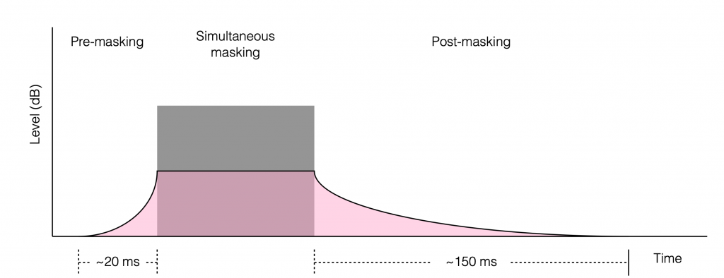
Fig 1. Generalised representation of temporal masking. The gray block is a loud noise. Anything in the pink area won’t be heard by most people most of the time. This plot is intentionally vague. The point is the effect, not the actual values.
So, if I were to play a loud noise (a gunshot, a blast of pink noise, a portion of an AC/DC song) and play a quiet sound before, during, or afterwards, and ask what the quiet sound was (to test if you heard it) your behaviour will match something like the plot in Figure 1. The gray block represents the loud sound. Anything in the pink shape is “stuff you can’t hear”. If the quiet sound occurs much earlier or much later than the loud sound, then it will have to be really quiet for you to not hear it. The closer in time the quiet sound occurs to the loud sound, the louder it has to be for you to hear it.
Of course, this is very general plot, so don’t use it for arguments while you’re drinking beer with your friends. For example, one element that I have not mentioned is frequency content. If the loud sound is the low frequency effects of a recording of distant thunder, and the quiet sound is a kitten mewing, then these two sounds are too far apart in frequency to have any influence on each other, and the graph is just plain wrong.
Signal Envelope
Unless you, like me, spend a lot of time listening to sinusoidal tones, you’ll notice that everything you listen to varies in level over time. This happens on different time scales. The sound pressure level (SPL) in the car while you’re driving to work or at the daycare picking up the kids is much louder than the SPL in your bedroom while you’re dealing with the free-floating existential anxiety that comes to visit at 2:00 in the morning. This is the ‘slow’ time scale. On the ‘fast’ end of the time scale, you have the extreme, and short SPL cause by closing a car door, or the very short, but not very loud sound of a high heel impacting a hardwood or tiled floor. Speech is somewhere in between these two. There are short, spikes caused by “t-” and “k-” sounds, and long-ish portions produced by vowels.
Note that we’re not really talking about how loud or how quiet things are. We’re talking about the change in level from quieter to louder and back again.
If we plot that change over time, we have a view of the signal’s envelope. For example, a single note on a piano has a fast attack (from quieter to louder) and a slow decay (from louder to quieter). A car horn honked in an open area (not a city intersection, where there are buildings to reflect the sound) has almost identical attack and decay envelopes.
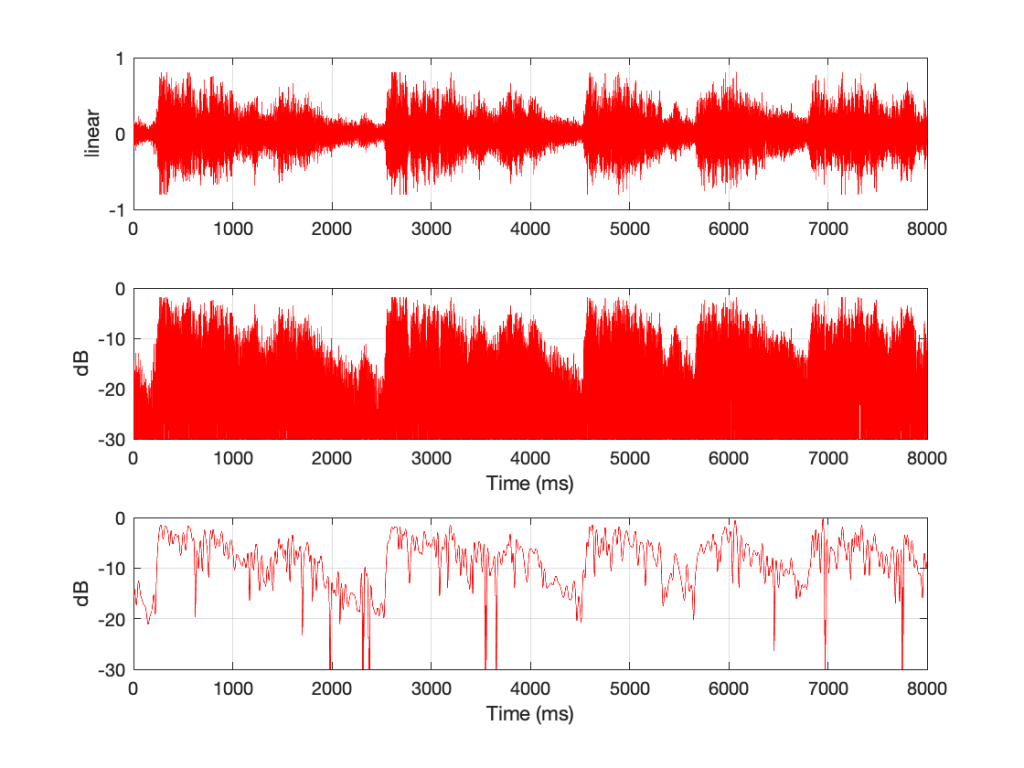
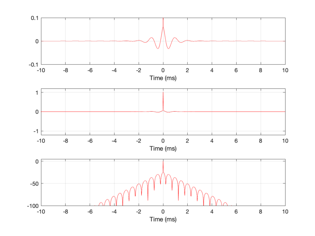
Fig 1. Three different representations of an audio signal in time.
Figure 1 shows an 8-second slice of a recording of the Alleluia Chorus from Handel’s “Messiah”, chosen because it’s easy for me to load that into Matlab using the “load handel” command, and I’m very lazy.
The top plot shows the signal in the way we’re used to looking at sound files. The x-axis is time, in ms. The Y-axis shows the linear value of each of the samples. Oddly, this is the way we normally look at sound files, but it represents how we hear sound very poorly, because we don’t hear amplitude linearly.
So, in the middle plot, I’ve taken the same data and, sample-by-sample, plotted each value on a decibel scale (using the equation DisplayOutput = 20*log10(abs(signal)). The absolute value is there because calculating the log of a negative number gives you strange results)
The third plot is the one we’re really interested in. That’s created by connecting the peaks in the middle plot, which results in a running plot of the signal’s level over time. This is its envelope. As you can see in that particular musical example, the attacks (the changes from quieter to louder) are steeper (and therefore faster) than the decays. This is not surprising. It’s hard to get an orchestra and choir to all stop instantaneously…
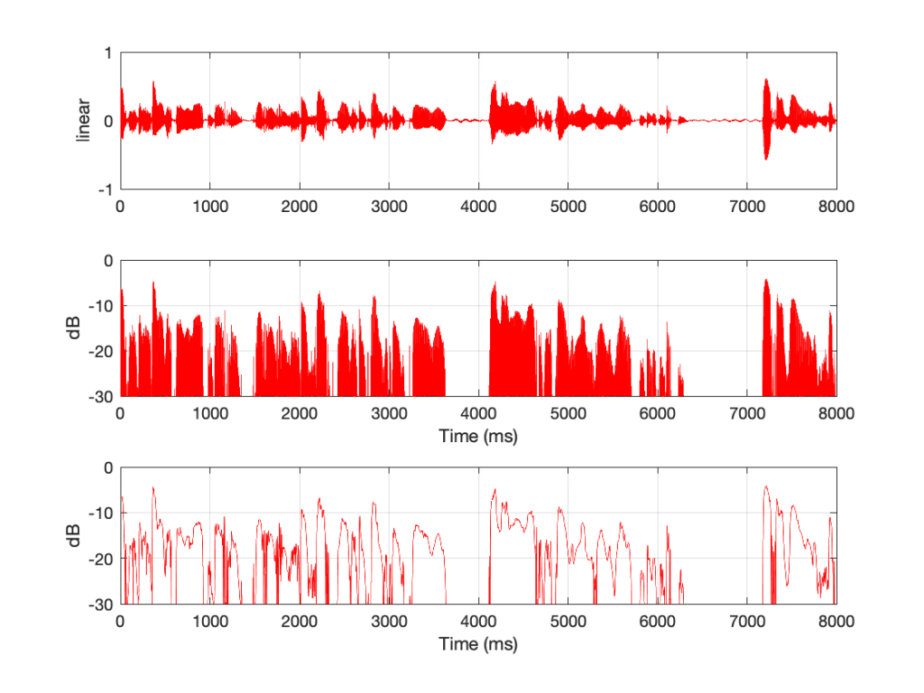
Fig 2. The same treatment to a different audio signal. In this case, it’s female speech recorded in an anechoic chamber.
Figure 2 shows the same three ways of plotting an audio signal, but in this case, the signal is female speech recorded in an anechoic chamber. Notice that, partly because it’s only one sound source and partly because there is no reverberation in the signal, the decays are almost as fast as the attacks. However, this is a very strange recording. Most people don’t listen to anything in an anechoic chamber, and we don’t typically go to the middle of a football field or a frozen lake to have a conversation.
Back to the “so what?”
Let’s assemble the three collections of information that we’ve been throwing around.
Firstly, focusing on filter response:
We know that filters can ring.
We also know that some filters can pre-ring.
We also know that, unless the Q is really high, that ringing decays pretty quickly.
Finally, we know that, if the frequency that’s ringing in the filter is not present in the signal, it won’t ring because there’s nothing there to ring. (Similarly if you turn up the low bass while listening to a solo piccolo recording, you won’t hear a difference because there’s no bass to boost.)
Secondly, we looked at our own response to quiet and loud signals in time
A loud sound will simultaneously mask a quiet sound that occurs at the same time (fancy-talk for “drown it out so I can’t hear it)
The loud sound will also post-mask a quiet sound that occurs after within a short time window (on the order of 100 – 200 ms)
The loud sound will also pre-mask a quiet sound that occurs before it within a short time window (on the order of 10 – 20 ms)
Finally, we looked at signal envelopes – the change in level of an audio signal over time
Sounds never start instantaneously. In order to do so, they would have to have an infinite frequency range measured at the receiver (e.g. your eardrum, which is most certainly band-limited as well). Even very fast attacks take milliseconds to ramp up.
Sounds in real life have longer decay times
I know, I know, you can name sounds that have very fast attacks (e.g. the pluck of a harpsichord plectrum on a high string, or a single xylophone bar struck in an anechoic environment) and very fast decays (ummm…. good luck finding something that decays more than 100 dB in less than 100 ms…)
The question is: if you have a filter that rings or pre-rings, and you apply it to a sound,
Is that ringing the thing that defines the envelope of the resulting sound? In other words, does the signal’s attack and/or decay envelope change significantly as a result of the time response of the filter?
Is that change in the envelope outside the limits of your ability to detect it due to pre-masking and post-masking?
There is no single answer to this question. If the audio signal is someone hitting a rim shot, and the filter is a peak filter with 12 dB of gain at 500 Hz with a Q of 100, then you’ll hear it ringing. In fact, it will sound like a rim shot with a sine wave generator. If the audio signal is a single bowed note on a ‘cello, and the filter is a dip filter with -3 dB of gain at 100 Hz with a Q of 0.707, then you won’t.
However, (for example) you CANNOT automatically jump to a conclusion that “pre-ringing sounds unnatural” because that starts with the assumption that you can hear it, and therefore it sounds “like” anything.
Whether or not you can hear the effects of a filter applied to an audio signal is dependent not only on the very specific characteristics of the filter, but its interaction with the signal. Change the filter OR change the signal, and the result will change.
This means that you CANNOT say things like “linear phase filters are better (or worse) than minimum phase filters” or “the pre-ringing of a linear phase filter sounds unnatural” because both of those statements start with the (possibly incorrect) assumption that you can hear the effect of the filter.
Now, don’t mis-interpret what I’ve said to mean “you can’t hear a filter ringing” – I didn’t say that. What I said was “just because a filter can be measured to be ringing doesn’t necessarily mean that you can hear it with a given audio signal”.
In this part, we’re going to do something a little weird.
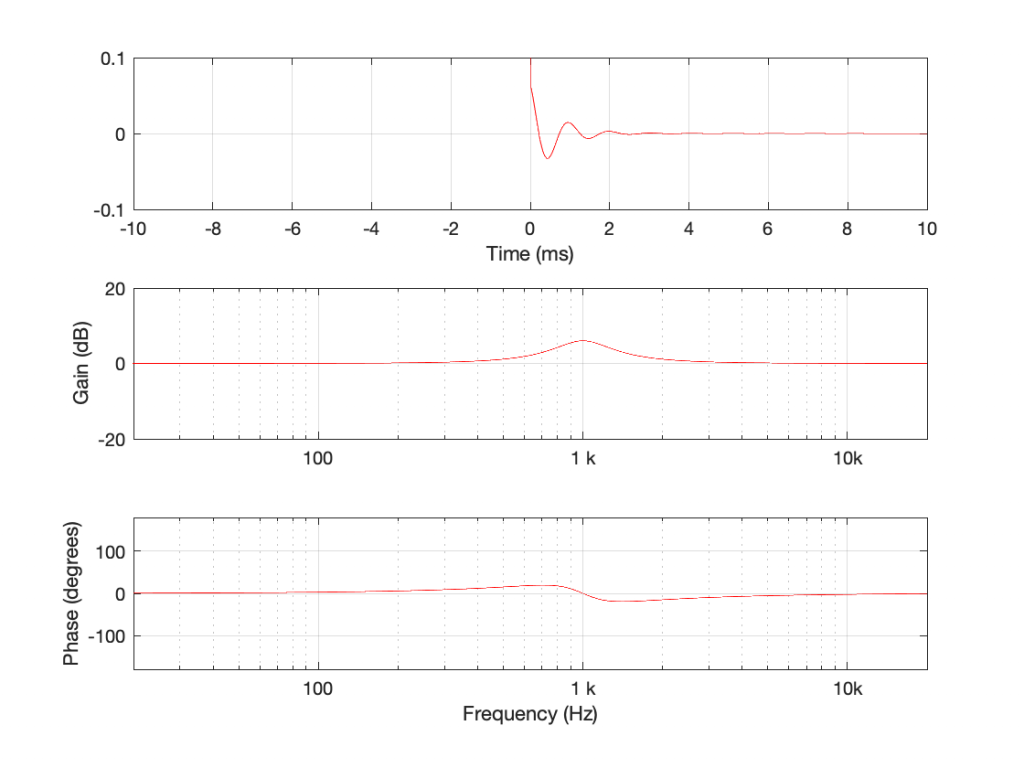
We’ll start by making a minimum phase peaking filter that has Q of 2 and a gain of +6 dB. The response of that filter is shown in Figure 1.
Fig 1. A minimum phase implementation of a peaking filter with a centre frequency of 1 kHz, a gain of 6 dB and a Q of 2.
Almost everything in the plots above should look familiar. The one weird thing is that I’ve left out the data in the time response before T = 0 ms. That’s because the future doesn’t matter, since we’re talking about a non-causal filter, right?
What if I (for some reason) wanted to make a filter that had a desired magnitude response, but a flat phase response? Let’s say that you’re allergic to phase shifts or you belong to an ancient religious cult that thinks that phase shifts are against the order of nature. How would we create that filter?
One way to do it is to create a filter that has the same magnitude response as the one above, but with an opposite phase response so that the two cancel each other. But, how do we create a filter with the opposite phase response?
One trick for doing this is to ignore what I said earlier. Remember when I was being pedantic about how filters advance signals in phase BUT NOT TIME? What if you were to ignore that for a brief moment? Could we use that ignorance to an advantage?
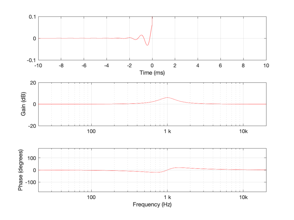
For example, what would happen if we took the time response shown above and reversed it? All of the component frequencies are still there, at all the same relative amplitudes. So the Magnitude Response won’t change. But what happens to the phase response? The answer is this:
Fig 2. The same impulse response as shown in Figure 1, reversed in time.
Now we have a weird filter that can only have an output based on future inputs (therefore it’s non-causal, and therefore not minimum-phase), with the same magnitude response as the one shown in Figure 1. But check out that phase response. It’s the inverse of the first filter.
So reversing time has the effect of flipping the polarity of the phase (not the polarity of the signal!) without modifying the magnitude response. What would have been a 45º phase shift (earlier) becomes a -45º phase shift (later).
So, if I were (conceptually – not really…) to put these two filters in series, feeding the output of one into the input of the other then their total magnitude responses would add (so I’d get a 12 dB boost instead of a 6 dB boost at 1 kHz) and their phase responses would cancel each other out. The end result would look like this:
Fig 3. The combination of the filters in Figure 1 and Figure 2. Notice that it has a gain of 12 dB at 1 kHz (because 6 + 6 = 12)
By now, you’ve probably figured out that what we’re looking at here is a linear phase filter, since can be used to change the magnitude response of a signal without mucking up its phase response.
The catch with this way of implementing a linear phase filter is that it has to see into the future. Of course, in real life this is difficult, but there is a trick you can use to fake it.
If you look at the impulse response plot in Figure 1, you can see that the peak in the response is at Time = 0 ms. As you get later, moving away from that moment in time, the signal is quieter and quieter until it dies away to (almost) nothing. The problem is that ‘almost nothing’ is not the same as ‘nothing’. In fact, if we’re being pedantic, the ringing keeps going forever, which is why it’s called a filter with an Infinite Impulse Response – an IIR filter.
This also means that the same is true for the filter in Figure 2, but the ringing extends infinitely backwards in time.
However, our resolution in measuring and storing the amplitude is not infinite – when the signal is quiet enough, we run out of resolution (‘ticks’ on the ruler) – and when the signal gets that quiet, it effectively becomes the same as nothing.
So, if we decide on the level where ‘almost nothing’ is the same as ‘nothing’ (this is more-or-less up to us if we’re the ones designing the filter), then we can look at the filter’s response and decide when that signal level is reached (both forwards and backwards in time).
For example, with the extremely limited resolution of the plots that I’ve made above, we can decide that ‘nothing’ is what’s left when you get ±10 ms from the impulse peak. Of course, the resolution of the pixels on that plot is not even close to the resolution of the audio signal, so ‘nothing’ on our plot and ‘nothing’ for the audio signal are two different things – but the concept is the same.
Back to the Future
Let’s pretend for a moment that, for the impulse response in Figure 3, we decide that ±10 ms is the window of time we need to get to ‘nothing’. This means that we could implement this filter by sending audio into it, letting it pre-ring with an increasing amount until it hits the maximum peak 10 ms after the sound comes into it, then ringing for another 10 ms until it’s out.
This means that the latency (the delay time between the input and the output of the filter) would appear to be 10 ms. Yes, when you feed in a signal, you immediately start getting something out of the filter, but the output is loudest after the signal has been feeding into the filter for 10 ms.
In other words, if you want to have a linear-phase filter that’s implemented using this method, you are going to have to accept that the cost will be latency. In our case (a filter with a Q of 2, with a centre frequency of 1 kHz, and the decisions we’ve made here) this results in a 10 ms latency. Change a parameter, and you change the latency. For example, as we’ve already seen, the lower the centre frequency, the longer in time the filter will ring. So, if we change the centre frequency of this filter to 100 Hz, then it will have 10 times the latency (because 100 Hz is 1/10 of 1 kHz – therefore the periodicity of the ringing is 10x longer). If we increase the Q, then the ringing lasts longer – both forwards and backwards and time.
Generally speaking, this means that, if you’re building a linear phase filter, you need to decide what characteristics the filter has, and then you need to start making decisions about the quality of the filter (e.g. is the response exactly what you want, or is just almost what you want?) and its latency.
Although I’m not going to talk about implementation much, the latency has two primary considerations. The first is obvious: are you willing to wait for the output? If you’re building a filter for a PA system, then you don’t want the output delayed so much that it sounds like an echo. However, the second issue is one for the person building the filter: latency means memory. This was a bigger problem in the ‘old days’ when memory was expensive, but it’s still an issue.
Why? The problem is that the latency is defined by the frequency and Q of the filter, which define the total time the filter takes to get through the entire impulse response. However, the filter’s processing doesn’t think of time in milliseconds, it thinks in samples. If you double the sampling rate, then you double the amount of memory you need to implement the filter.
So, going from 48 kHz to 192 kHz requires 4x the memory.
A little perspective
One thing to notice in the three figures above is the vertical scale of the time response plots. You can see there that the range is ±0.1, which is a zoomed-in view of the amplitude. This may give you a distorted impression of the level of the ringing relative to the signal (the impulse). Figure 4 should clear this up.
Fig 4. Three plots showing exactly the same data in three different ways.
The top plot in Figure 4 is identical to the top plot in Figure 3. The middle plot is also on a linear amplitude scale, but the range of the plot shows the entire range of the signal. You can see there that the impulse at T = 0 hits a value of 1, and so the pre- and post-ringing isn’t as loud as you might have thought based on the first three figures.
The bottom plot shows the same information, plotted on a dB scale instead. The impulse at T = 0 ms hits 0 dB. Relative to that, the pre- and post-ringing has a maximum value of about -24 dB. You can also see there that the ringing is at least 100 dB down by the time we’re 6 ms away from the main impulse, looking both backwards and forwards in time.
Of course, all of these characteristics would be different for filters with different parameters. The point here is to understand the general characteristics, not the specifics.
Additional Comment
You may read on various fora someone who claims that there’s no such thing as “pre-ringing”. “It’s ‘ripple'” They’ll claim.
This is incorrect.
Pre-ringing and ringing are behaviours that occur in the time domain.
Ripple is a wiggle in the response in the frequency domain. (Say, for example, you zoom into the magnitude response, it won’t be completely flat in some cases – and if it’s not, you have ripple.)