Part 1
Part 2
Part 3
Part 4
Part 5
Part 6
Part 7
Part 8a
Part 8b
We’ve already seen that nothing can exist in the audio signal above the Nyquist frequency – one half of the sampling rate. But that’s the audio signal, what happens to filters? Basically, it’s the same – the filter can’t modify anything above the Nyquist frequency. However, the problem is that the filter doesn’t behave well to everything up to the Nyquist and then stop, it starts misbehaving long before that…
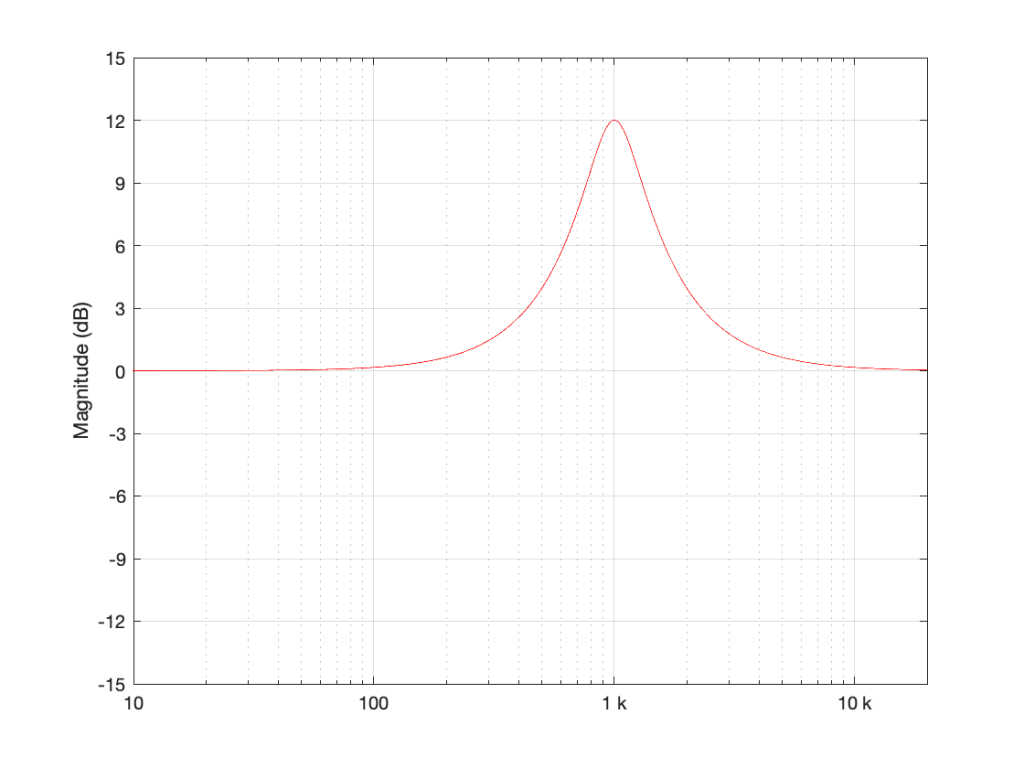
Let’s make a simple filter: a peaking filter where Fc=1 kHz, Gain = 12 dB, and Q=1. The magnitude response of that filter is shown in Figure 1.
What happens if we implement this filter with a sampling rate of 48 kHz and 192 kHz, and then look at the difference between the two? This is shown in Figure 2.
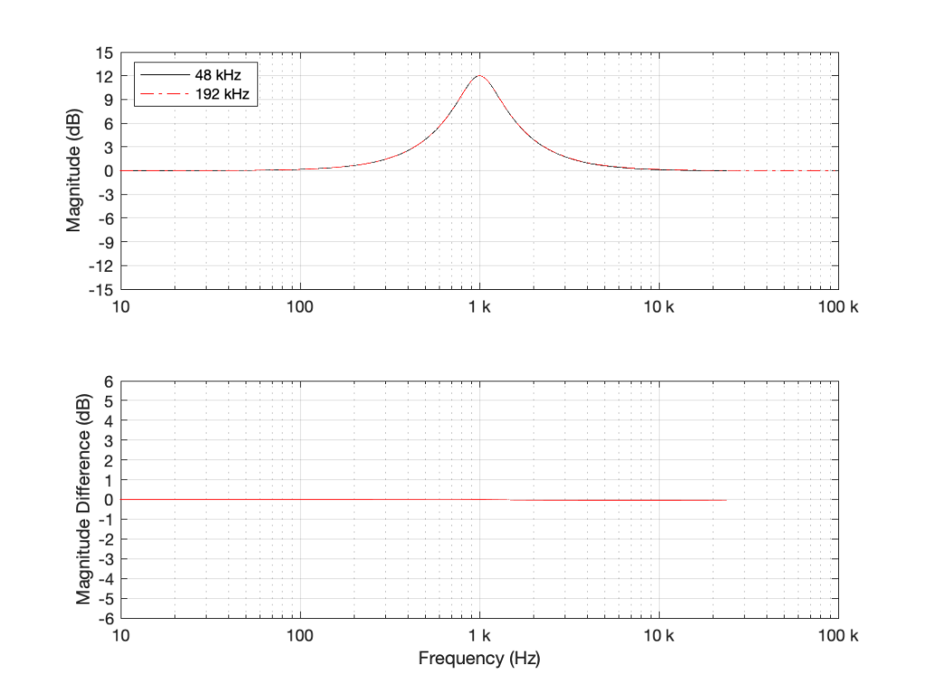
As you can see in Figure 2, the filter, centred at 1 kHz, is almost identical when running at 48 kHz and 192 kHz. So far so good. Now, let’s move Fc up to 10 kHz, as shown in Figure 3.
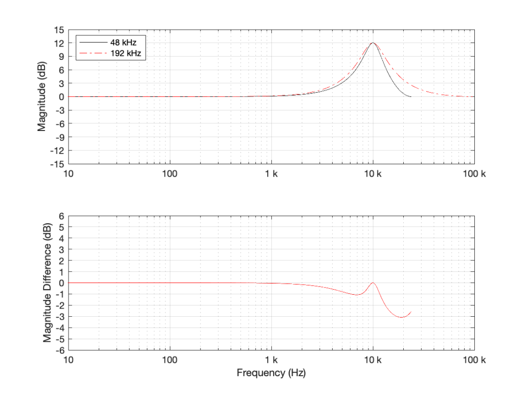
Take a look at the black plot on the top of Figure 3. As you can see there, the 48 kHz filter has a gain of 0 dB at 24 kHz – the Nyquist frequency. Looking at the red dotted line, we can see that the actual magnitude of the filter should have been more than +3 dB. Also, looking at the red line in the bottom plot, which shows the difference between the two curves, the 48 kHz filter starts deviating from the expected magnitude down around 1 kHz already.
So, if you want to implement a filter that behaves as you expect in the high frequency region, you’ll get better results easier with a higher sampling rate.
However, do not jump to the conclusion that this also means that you can’t implement a boost in high frequencies. For example, take a look at Figure 4, which shows a high shelving filter where Fc = 1 kHz, Gain = 12 dB and Q = 0.707.
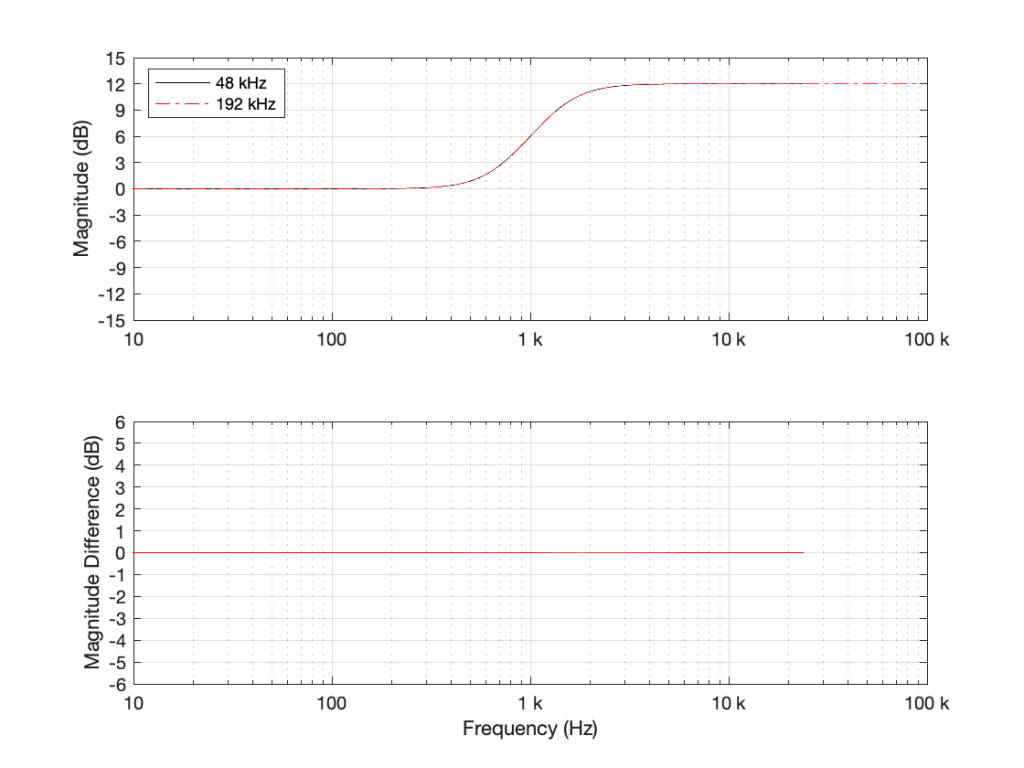
As you can see in the bottom plot in Figure 4, the two filters in this case (one running at 48 kHz and the other at 192 kHz) have almost identical magnitude responses. (Actually, there is a small difference of about 0.013 dB…) However, if the Fc of the shelving filter moves to 10 kHz instead (keeping the other two parameters the same) then things do get different.
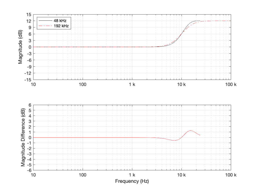
As can be seen there, there is a little over a 1 dB difference in the two implementations of the same filter.
Some comments:
- I’m not going to get into exactly why this happens. If you want to learn about it, look up “bilinear transform”. The short version of the issue is that these filters are designed to work in a system with an infinite sampling rate and bandwidth (a.k.a. analogue), but the band-limiting of an LPCM digital system makes things misbehave as you get near the Nyquist frequency.
- This does not mean that you cannot design a filter to get the response you want up to the Nyquist frequency.
If you look at the red dotted curve in Figure 3 and call that your “target”, it is possible to build a filter running at 48 kHz that achieves that magnitude response. It’s just a little more complicated that calculating the gain coefficients for the biquad and pretending as if you were normal. However, if you’re a DSP Engineer and your job is making digital filters (say, for correcting tweeter responses in a digitally active loudspeaker, for example) then dealing with this issue is exactly what you’re getting paid for – so you don’t whine about it being a little more complicated. - The side-effect of this, however, is that, if you’re a lazy DSP engineer who just copies-and-pastes your biquad coefficient equations from the Internet, and you just plug in the parameters you want, you aren’t necessarily going to get the response that you think. Unfortunately, this is not uncommon, so it’s not unusual to find products where the high-frequency filtering measures a little strangely, probably because someone in development either wasn’t meticulous or didn’t know about this issue in the first place.