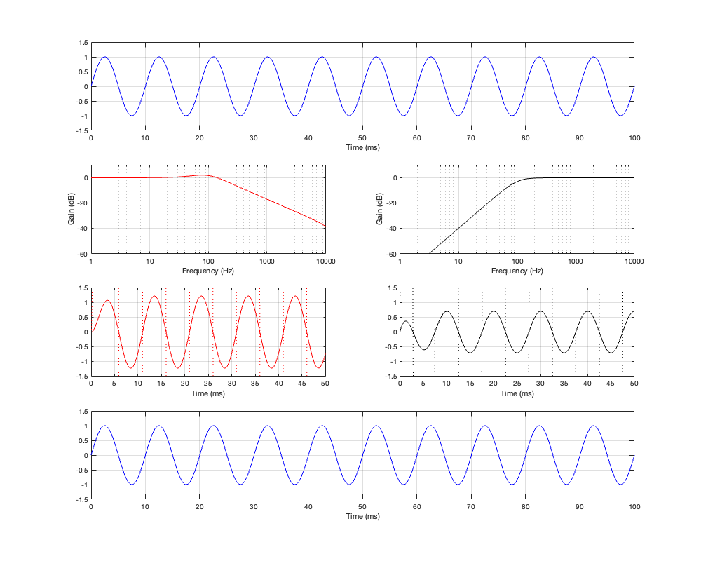
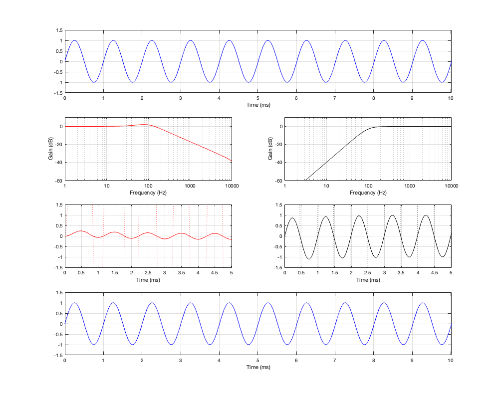
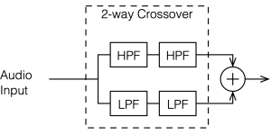
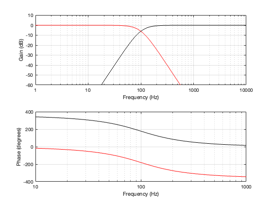
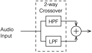
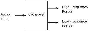
Up to now, we’ve been looking at two-way crossovers with different implementation types, analysing the responses of the two individual outputs and the total summed output as if we just mixed the two frequency bands electrically. This analysis shows us what the crossover does in isolation, but this is just a small portion of what’s happening in real life.
Let’s now start by including some real-world implications into the mix to see what happens.
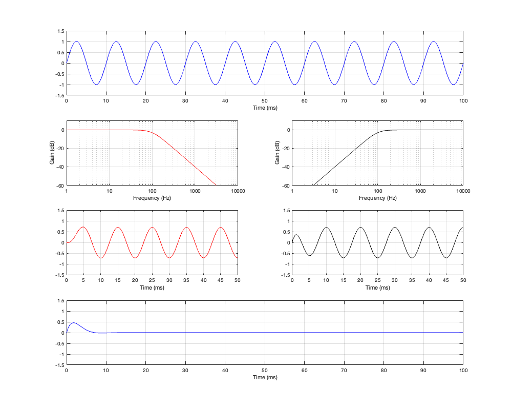
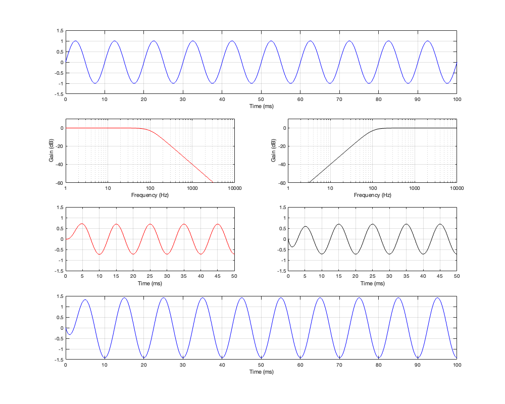
For this posting, I won’t be just adding the two outputs of the high- and low-pass filter paths. We’re now going to pretend that the outputs of those two paths are connected to two point-source loudspeakers floating in infinite space. Since they’re both point sources, each one has a flat magnitude response and a flat phase response relative to its input, and these two characteristics are true in all directions. They also have no frequency limits. So, although I’m calling one a “tweeter” and the other a “woofer”, they don’t behave like real loudspeakers.
Using this kind of model allows me to analyse the implications of the differences in distances to the microphone (or listening) position, including the characteristics of the crossover.
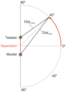
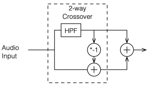
Figure 6.1 shows a schematic diagram of the system that we’re analysing in this posting. As you ca see, the “tweeter” and “woofer” are separated by some vertical distance. The microphone position is at some distance from the centre of the two loudspeakers (the radius of the big semi-circle in the drawing), and at some angle above or below the on-axis angle to the loudspeaker pair. In my analyses, negative angles are below the horizon, and positive angles are above.
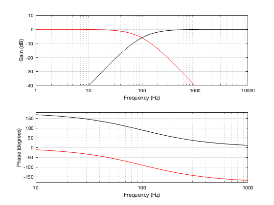
If the angle is 0º, then the distances to the tweeter and the woofer are identical, and the result is the same as the plots I’ve shown in Parts 2, 3, 4, and 5. However, if the angle to the microphone goes positive, then this means that the woofer’s signal will be delayed relative to the tweeter’s, and this will have some effect on the way the two signals interfere with each other when they are summed.
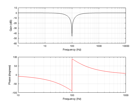
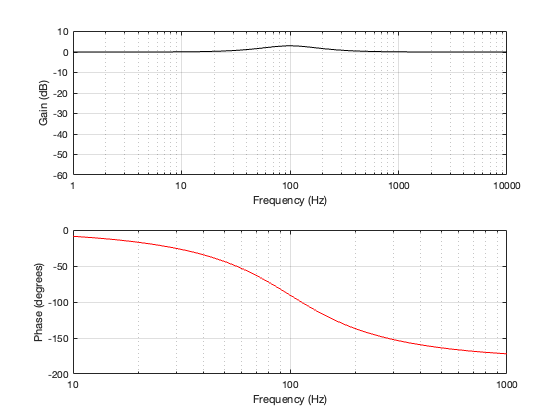
This change in interference results in a change in the magnitude response of the summed signals at the microphone as a function of the angle. So, another way to consider this is that we’re changing the directivity of the loudspeaker pair.
For all of the plots below, I’ve shown the responses at angles in 30º increments from -90º to 90º. As I’ve said above, the 0º plot should be identical to the plot for the same crossover type shown in one of the previous postings.
Of course, a change in the separation between the two drivers will change the amount of effect on the magnitude response when the angle to the microphone is not 0º. For these plots, I’ve decided to keep the crossover frequency at 100 Hz, to maintain consistency, and to plot the responses for 3 example loudspeaker separations: 43.125 cm (0.125 * wavelength at 100 Hz), 86.25 cm (0.25 * wavelength at 100 Hz), and 1.725 m (0.5 * wavelength at 100 Hz).
The point of these is not really to give “real world” suggestions, but to show tendencies…
2nd-order Butterworth
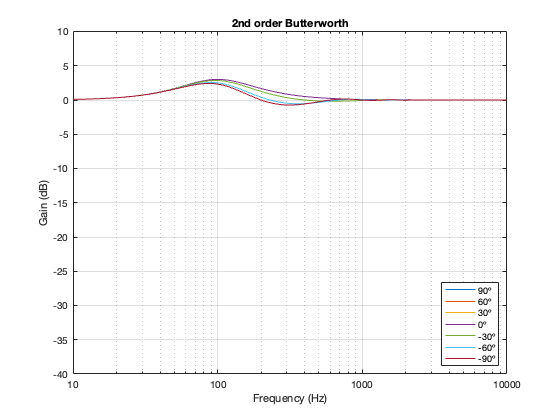
Separation = 0.125 * wavelength at 100 Hz
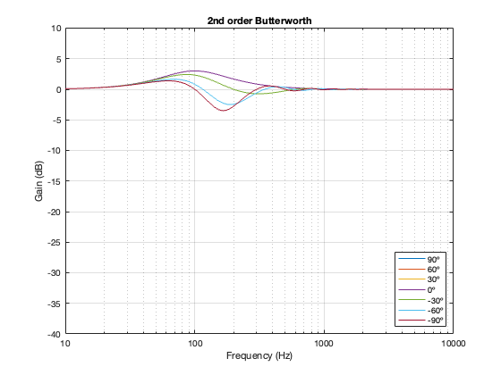
Separation = 0.25 * wavelength at 100 Hz
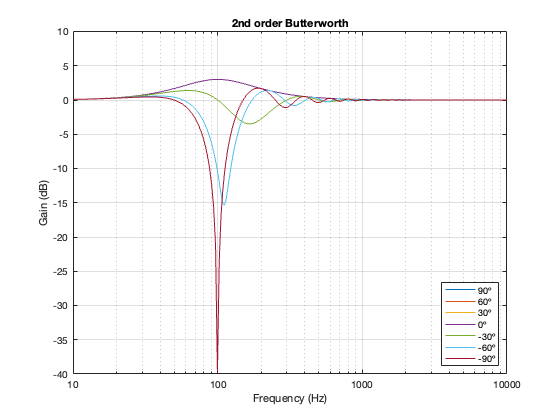
Separation = 0.5 * wavelength at 100 Hz
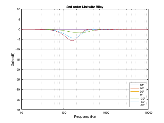
Not surprisingly, the greater the separation between the loudspeaker drivers, the bigger the effect on the magnitude response off-axis. Notice, however, that the effect is not symmetrical. In other words, the magnitude responses at -90º and 90º are not the same. This is because the relative phase responses of the two filter paths (also remembering that the tweeter’s signal is flipped in polarity) has an effect on the sum of the two signals at different points in space.
Hopefully, it’s clear that if the crossover had been at a different frequency, the characteristics of the magnitude responses would have been the same – they would have just moved in frequency. This is because I’m relating the separation between the two loudspeaker drivers as a fraction of the wavelength of the crossover frequency.
And, of course, you don’t need to email me to remind me that a loudspeaker separation of 1.725 m is silly. As I said, the point of this is NOT to help you design a loudspeaker, it’s to show the characteristics and the tendencies. (On the other hand, 1.725 m between a subwoofer and a main loudspeaker is not silly… so there…)
4th-order Linkwitz Riley
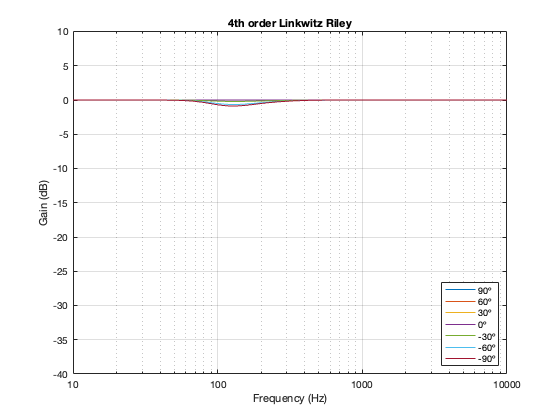
Separation = 0.125 * wavelength at 100 Hz
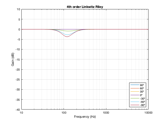
Separation = 0.25 * wavelength at 100 Hz
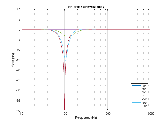
Separation = 0.5 * wavelength at 100 Hz
Notice here that the magnitude responses never go above 0 dB at any angle. It’s also interesting that at smaller separations, the difference in the magnitude response as a function of angle is smaller than that for the 2nd-order Butterworth crossover.
2nd-order Linkwitz Riley
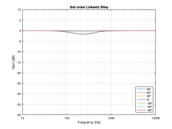
Separation = 0.125 * wavelength at 100 Hz
Separation = 0.25 * wavelength at 100 Hz
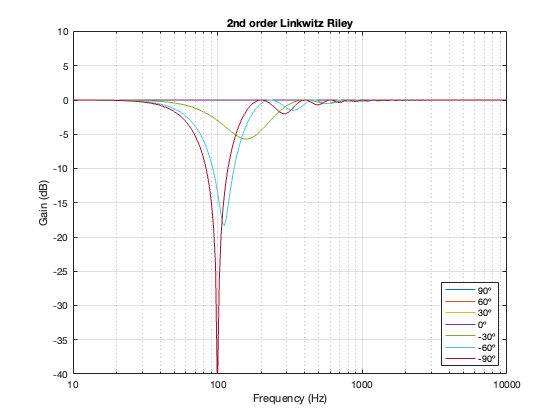
Separation = 0.5 * wavelength at 100 Hz
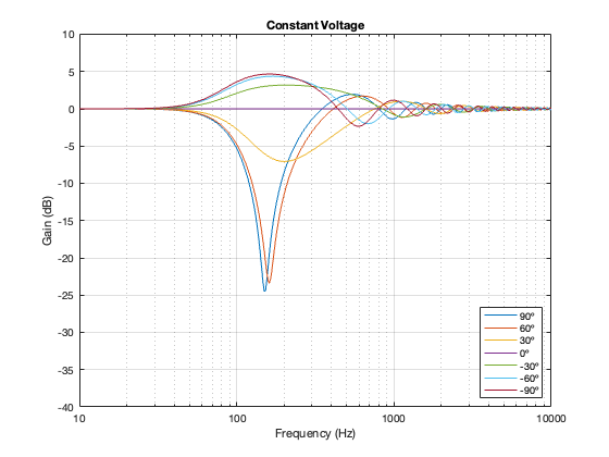
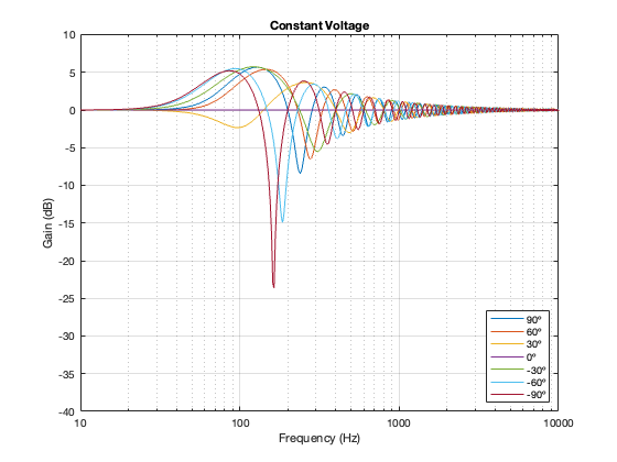
Constant Voltage
As I mentioned in the previous posting, there are many ways to implement a constant voltage crossover. The plots below show analyses of the same crossover as the one I shows in Part 5 – using a 2nd-order Butterworth for the high-pass section, and subtracting that from the input to create the low-pass section.
Separation = 0.125 * wavelength at 100 Hz
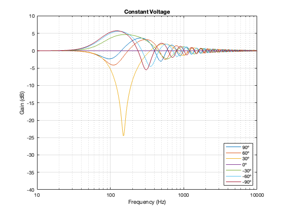
Separation = 0.25 * wavelength at 100 Hz
Separation = 0.5 * wavelength at 100 Hz
One thing to notice here is that, although we saw in Part 5 that a constant voltage crossover’s output is identical to its input, that’s only true for the hypothetical example where we just summed the outputs. You’ll notice that, at a microphone angle of 0º in this still-hypothetical example, the total magnitude response is still flat. However, at other angles, the change in magnitude response is much larger than it is for the other crossover types for angles between -60º and 60º. Therefore, if you jumped to the conclusion in the previous posting that a constant voltage design is the winner, you might want to re-consider if you don’t live in a room that extends to infinite space without any walls (or a perfect anechoic chamber), and you only listen on-axis to the loudspeaker.
Just sayin’…
P.S.
In case you’re wondering, it’s also possible to look at the effects of summing the outputs of the two loudspeakers without including a crossover in the signal path. The result of this is that you have two full-range drivers, whose only difference at the microphone position is the time of arrival as a function of the angle of the microphone relative to the “horizon”. This results in two big differences in what you see above:
- The total output when the interference is construction is + 6 dB relative to the input. This happens because the two signals are identical, and, at some frequencies and some microphone positions, they just add together.
- The interference extends to a much wider frequency band, since both loudspeakers’ signals are interfering with each other at all frequencies.
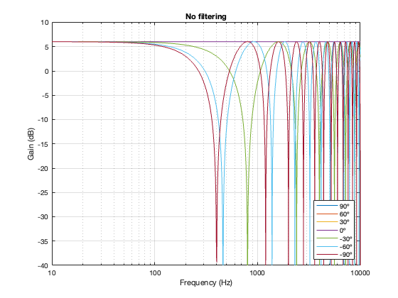
Separation = 0.125 * wavelength at 100 Hz
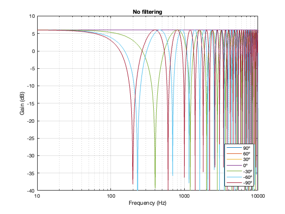
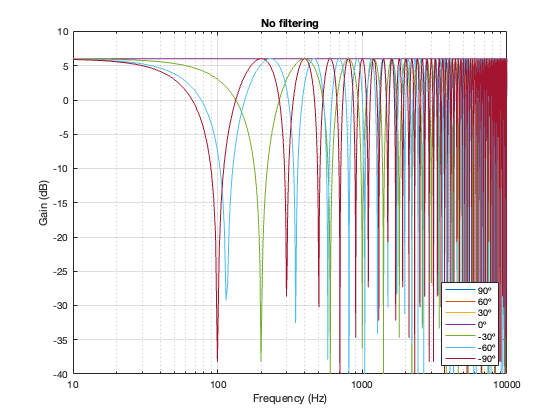
Figure 6.16. No crossover
Separation = 0.5 * wavelength at 100 Hz