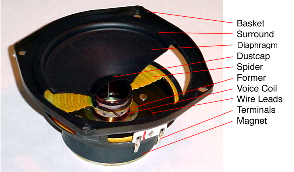
Let’s look at a typical moving coil loudspeaker driver like the woofer shown in Figure 1.
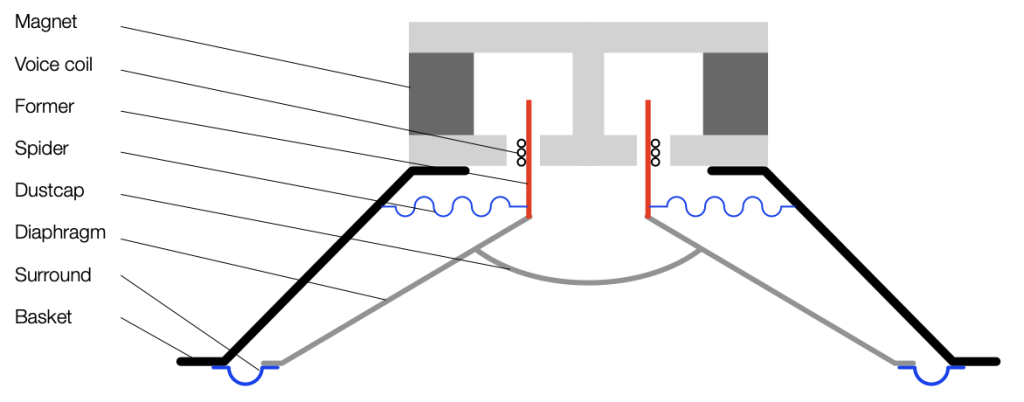
If I were to draw a cross-section of this and display it upside-down, it would look like Figure 2.
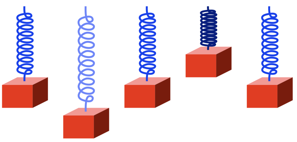
Typically, if we send a positive voltage/current signal to a driver (say, the attack of a kick drum to a woofer) then it moves “forwards” or “outwards” (from the cabinet, for example). It then returns to the rest position. If we send it a negative signal, then it moves “backwards” or “inwards”. This movement is shown in Figure 3.
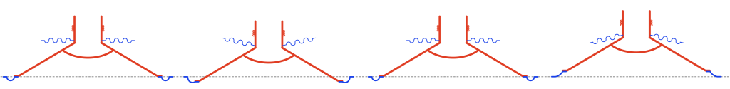
Notice in Figure 3 that I left out all of the parts that don’t move: the basket, the magnet and the pole piece. That’s because those aren’t important for this discussion.
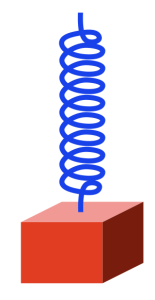
Also notice that I used only two colours: red for the moving parts that don’t move relative to each other (because they’re all glued together) and blue for the stretchy parts that act as a spring. These colours relate directly to the colours I used in Part 1, because they’re doing exactly the same thing. In other words, if you hold a woofer by the basket or magnet, and tap it, it will “bounce” up and down because it’s just a mass suspended by a spring. And, just like I talked about in Part 1, this means that it will oscillate at some frequency that’s determined by the relationship of the mass to the spring’s compliance (a fancy word for “springiness” or “stiffness” of a spring. The more compliant it is, the less stiff.) In other words, I’m trying to make it obvious that Figure 3, above is exactly the same as Figures 3 and 5 in Part 1.
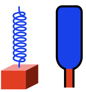
However, it’s very rare to see a loudspeaker where the driver is suspended without an enclosure. Yes, there are some companies that do this, but that’s outside the limits of this discussion. So, what happens when we put a loudspeaker driver in a sealed cabinet? For the purposes of this discussion, all it means is that we add an extra spring attached to the moving parts.
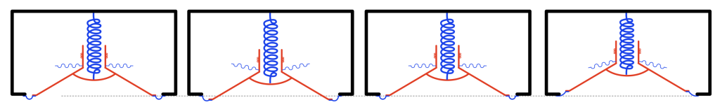
I’ve shown the “spring” that the air provides as a blue coil attached to the back of the dust cap. Of course, this is not true; the air is pushing against all surfaces inside the loudspeaker. However, from the outside, if you were actually pushing on the front of the driver with your fingers, you would not be able to tell the difference.
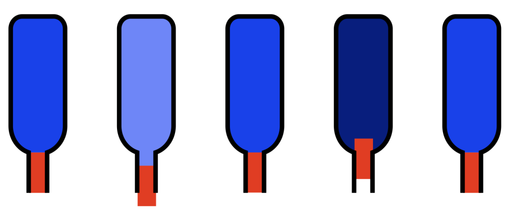
This means that the spring that pushes or pulls the loudspeaker diaphragm back into position is some combination of the surround (typically made of rubber nowadays), the spider (which might be made of different things…) and the air in the sealed cabinet. Those three springs are in parallel, so if you make one REALLY stiff (or lower its compliance) then it becomes the important spring, and the other two make less of a difference.
So, if you make the cabinet too small, then you have less air inside it, and it becomes the predominant spring, making the surround and spider irrelevant. The bigger the cabinet, the more significant a role the surround and spider play in the oscillation of the system.
Sidebar: If you are planning on making a lot of loudspeakers on a production line, then you can use this to your advantage. Since there is some variation in the compliance of the surround and spider from driver-to-driver, then your loudspeakers will behave differently. However, if you make the cabinet small, then it becomes the most important spring in the system, and you get loudspeakers that are more like each other because their volumes are all the same.
Remember from part 1 that if you increase the stiffness of the spring, then the resonant frequency of the oscillation will increase. It will also ring for longer in time. In practical terms, if you put a woofer in a big sealed cabinet and tap it, it will sound like a short “thump”. But if the cabinet is too small, then it will sound like a higher-pitched and longer-ringing “bonnnnnnnggggg”.
So far, we’ve only been talking about physical things: masses and springs. In the next part, we’ll connect the loudspeaker driver to an amplifier and try to push and pull it with electrical signals.