Part 1
Part 2
Part 3
Part 4
Part 5
Part 6
Back in Part 5 of this series, I described an example of a pretty typical / normal signal flow for an audio signal that you’re playing from a streaming service to a “smart-ish” loudspeaker in your house. If you read through that list, you’ll see that I mentioned that the signal might be sampling-rate converted two times (once in your player, and once again in your loudspeaker or headphones).
Let me say something very clearly, before we go any further:
- There’s no guarantee that this is happening.
For example, many players don’t sampling-rate convert the signal if the device they’re sending the signal is compatible with the sampling rate of the signal. However, many players do sampling-rate convert the signal – and many devices (like DACs, for example) are not compatible with all sampling rates, so the player is forced to do something about it. - Sampling rate conversion is not necessarily a bad thing.
There are many good sampling rate converters out there in the world. In fact, you can use a high-quality sampling rate converter to reduce problems with jitter coming in from an “upstream” device or transmission path.
However, sampling rate conversion is not necessarily a good thing either… so the more of them you have in your audio signal path, the better you want them to be. In an optimal case, the artefacts caused by the sampling rate converter will not be the “weakest link” in the audio chain.
However, this last statement is very easy to mis-interpret, as I alluded to in Part 6. The problem is that, if I say “I have a sampling rate converter with a THD+N of -100 dB relative to the signal level” this might look pretty good. However, if the signal and the SRC artefacts are in COMPLETELY different frequency bands, and you’re playing the signal out of a loudspeaker that can’t produce the signal (say, because it’s too low in frequency) then 100 dB might not be nearly good enough. In other words, it’s not a mere numbers-game… you have to know how to interpret the data…
A what?
Maybe we should first back up a little and talk about what a sampling rate converter is. As you saw in Part 1, at its most basic level, LPCM digital audio is just a way of describing a signal by storing a long string of measurements that were made at a regular time interval. Each of those measurements is called a “sample” and the rate at which you measure the samples (per second) is called the “sampling rate”. A CD, for example, uses a standard sampling rate of 44,100 samples per second, or 44.1 kHz. Other systems use other rates.
If you want to listen to a CD on a loudspeaker with built-in digital processing, and the loudspeaker happens to have an internal sampling rate that is NOT 44.1 kHz (let’s say that it’s 48 kHz), then you need to somehow convert the sampling rate from 44.1 kHz to 48 kHz to get things to work properly. (This is a little like having a gearbox in a car – your engine does not turn at the same speed as your wheels – you put gears in-between to convert the rotational speed of the engine to the rotational speed of the wheels.)
One sneaky way to do this is to use an analogue connection – you convert the 44.1 kHz digital signal to an analogue one using a DAC, and then re-sample the analogue signal using an ADC running at 48 kHz. This is simple, and (if you choose your DAC and ADC properly) potentially a really good solution. In the “old days” (up to the 1990s) before digital SRCs became really good, this was the best way to do it (assuming you had access to some decent gear).
There are many ways to make a fully-digital SRC. For example:
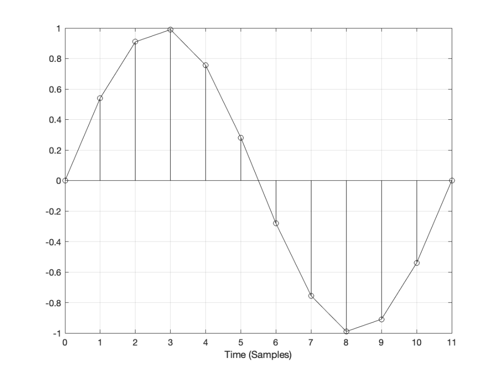
Let’s say that you have an audio signal that’s been sampled at some sampling rate that we’ll call “Fs1” (for “Sampling Frequency 1”) , as is shown in Figure 1.
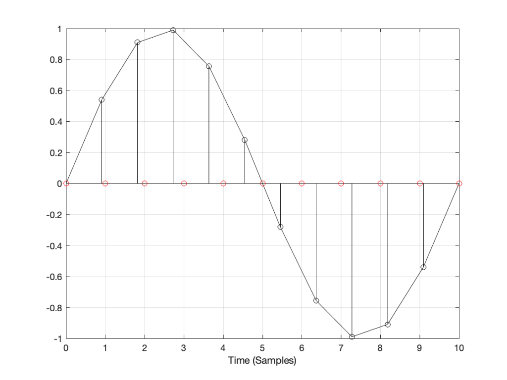
You then want to have the same signal, represented at a different sampling rate, which we’ll call Fs2. The old signal (in black) and the new sampling rate (the red dots and the gridlines) can be seen in Figure 2.
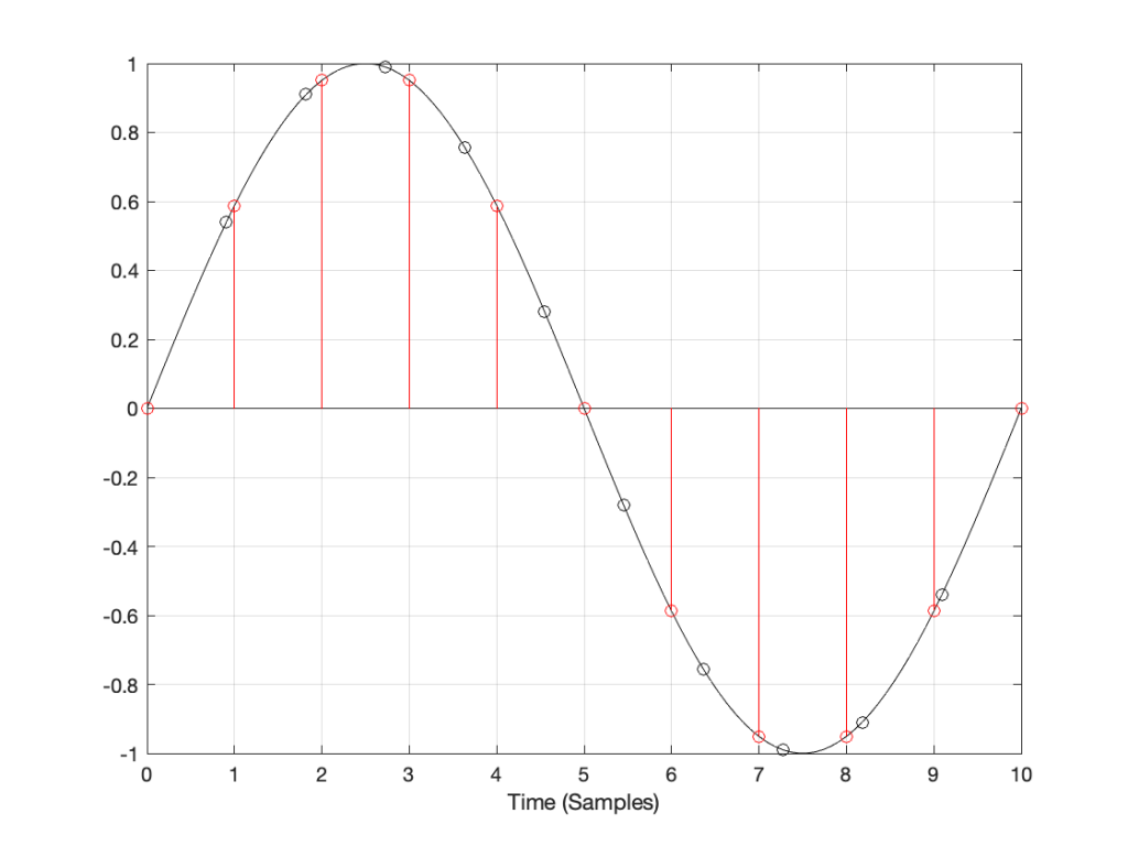
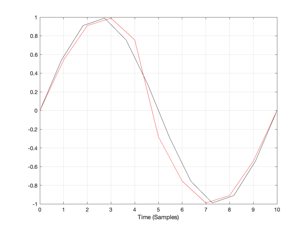
How do we do this? One way is to draw straight lines between the original samples, and calculate the values at the point on the line that corresponds with the time of the new samples. This is called “linear interpolation” (because it’s based on drawing straight lines between the original samples), and it’s shown in Figure 3.

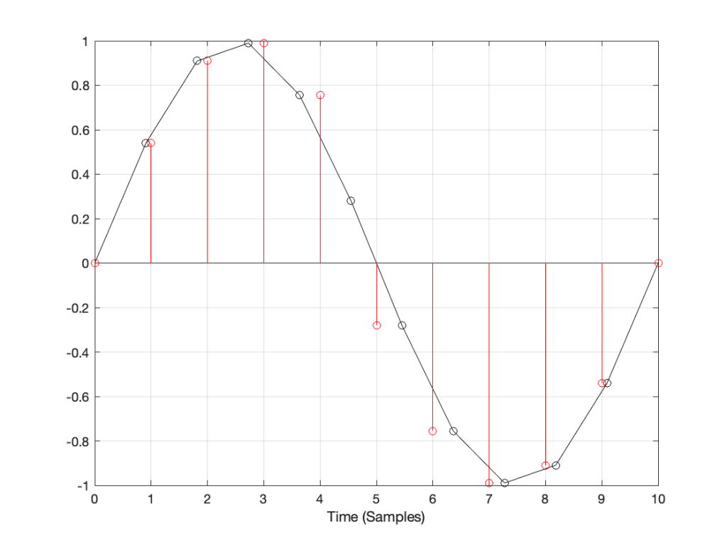
A better way to do this is to use some fancy math to calculate where the signal would be after the reconstruction filter smoothed it back to the original (band-limited) input. There are different ways to do this (in other words, different mathematical strategies) that are outside the scope of this posting, however, I’ve shown an example of a piecewise cubic spline interpolation implementation in Figure 4, below.
However, let’s say that:
- you’ve been given the job of building a sampling rate converter, but
- you think that the examples I gave above are way to complicated…
What do you do? One possibility is to look at the sample value that you want to output, find the closest sample (in time) in the original signal, and use that. This is a technique commonly called “nearest neighbour” for obvious reasons – and it’s one of the worst-performing SRC strategies you can use. An example of this is shown in Figure 5, below. Notice that the new values (the red circles) are identical to the closest original value
If we look at these two signals without the sample values, we’ll see some pretty nasty distortion in the time domain, as shown in Figure 6.
So what?
The plots above show the results of good and bad SRCs in the time domain, but what does this look like in the frequency domain? Let’s take a couple of specific examples.

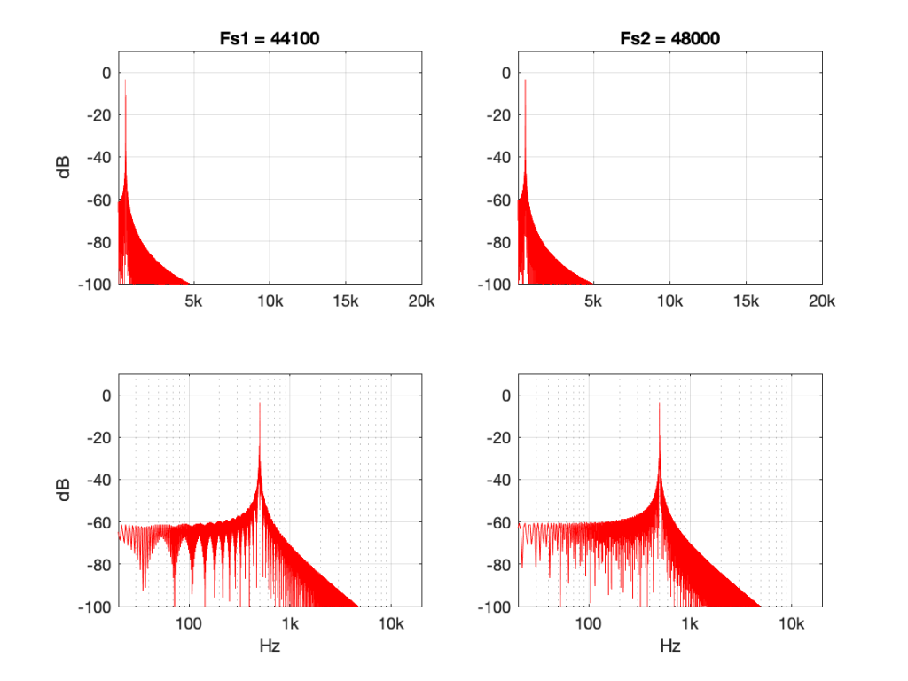
Figures 7 and 8 look almost identical. There are the windowing artefacts of the frequency analysis that I’m doing are larger than most of the artefacts caused by the interpolation implementations. However, you may notice a couple of spikes sticking up between 1 kHz and 10 kHz in Figure 7. These are the most obvious frequency-domain artefacts of the distortion caused by linear interpolation. Notice however, that those artefacts are about 80 dB down from the signal – so that’s pretty good for a cheap implementation.
However, let’s look at the same 500 Hz tone converted using the “nearest neighbour” strategy.
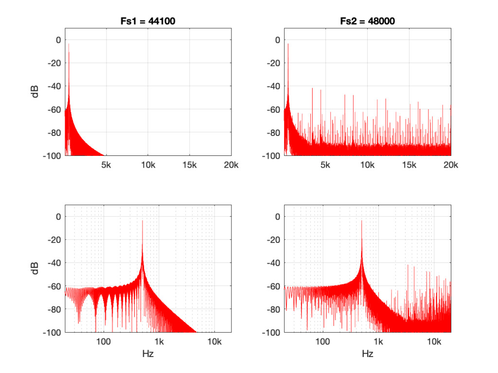
Now you can see that things have really fallen apart The artefacts are almost up to 40 dB below the signal level, and they’re quite far away in frequency, so they’ll be easy to hear. Also remember that the artefacts that are generated here are inside the audio band, so they will not be eliminated later in the chain by a reconstruction filter in a DAC, for example. They’re there to stay.
There’s one more interesting thing to consider here. Let’s try the same nearest neighbour algorithm, converting between the same two sampling rates, but I’ll put in signals at different frequencies.
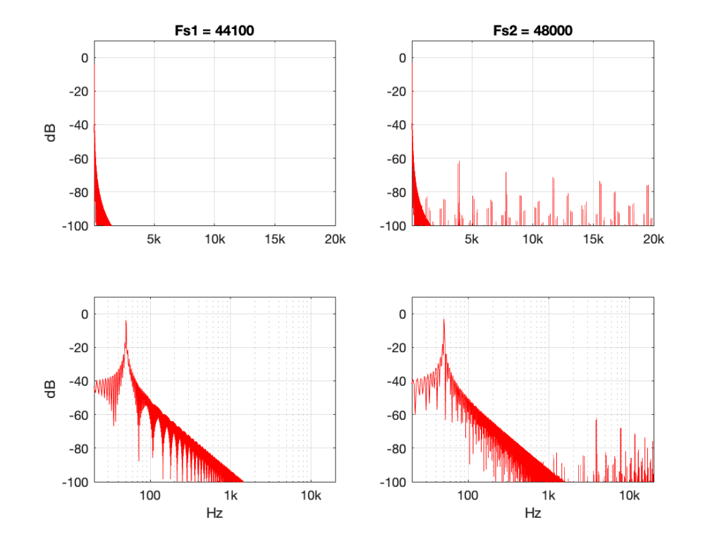
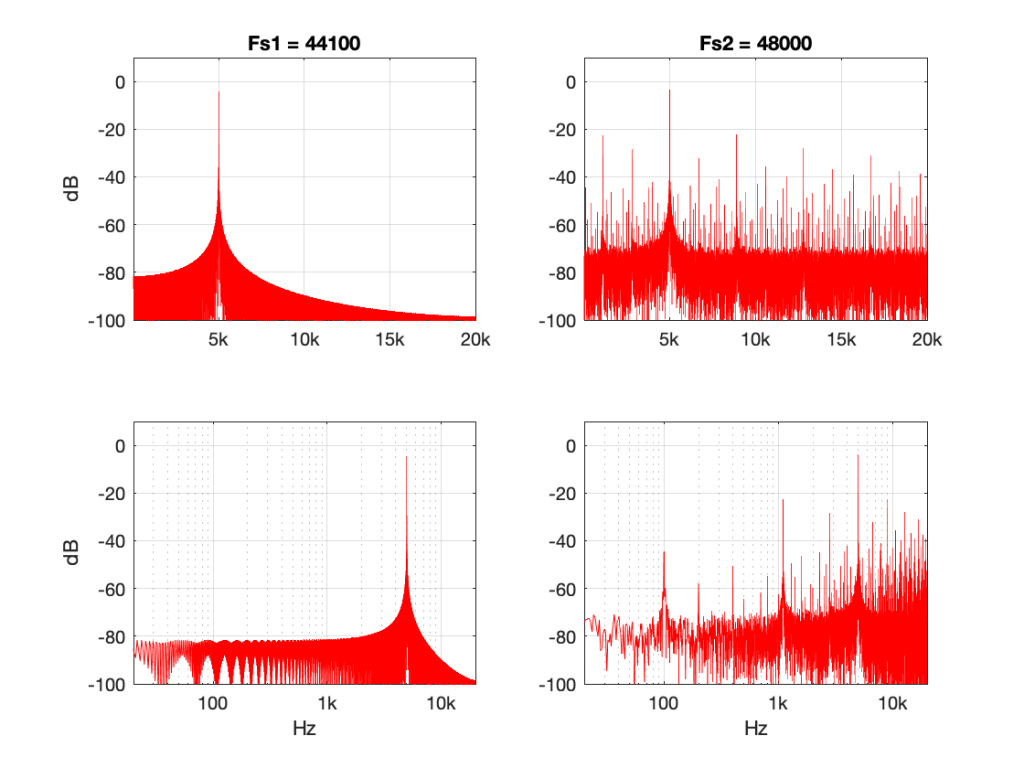
Figure 10 shows the same system, but the input signal is a 50 Hz sine wave (instead of 500 Hz). Notice that the artefacts are now about 60 dB down (instead of 40 dB).
Figure 11 shows the same system again, but the input signal is a 5 kHz sine wave. Notice that the artefacts are now only about 20 dB down.
So, with this poor implementation of an SRC, the distortion-to-signal ratio is not only dependent on the algorithm itself, but the signal’s frequency content. Why is this?
Think back to the way the “nearest neighbour” strategy works. You’re simply copying-and-pasting the value of the nearest sample. However, the lower the frequency, the less change there is in the signal from sample to sample. So, as your signal’s frequency goes down (more accurately, as it gets further away from the sampling rate), the smaller the error that you create with this system. At 0 Hz, there would be no error, because all of the samples would have the same value.
So, (for example) if your job is to build the SRC in the first place, and you measure it with a 50 Hz tone, you’ll see that the artefacts are 60 dB below the signal and you’ll pat yourself on the back and go to lunch. Then, some weeks later, when the customer complaints start coming in about tweeter distortion, you’ll think it must be someone else’s fault… but it isn’t…
Conclusion
What does this have to do with “High Resolution Audio”? Well, the problem is that most audio gear does not run at crazy-high sampling rates (this is not necessarily a bad thing), so if you play a high-res file, you’re probably sampling rate converting (this is not necessarily a bad thing).
However, if your gear does have a bad SRC in the signal flow (and, yes, this is not uncommon with modern audio gear) then you either need to
- play the signal with a different (e.g. not-high-res) sampling rate to find out if it’s better,
OR - buy better gear,
OR - at least check for a firmware update.
Note that first recommendation of the three: Because the quality of a sampling rate converter is very dependent upon the relationship between the input and the output sampling rates, it can happen that a “normal” resolution audio signal (say, at 44.1 kHz) will sound better on your particular equipment than a “high” resolution audio signal (say, at 192 kHz) because of this. Of course, the opposite could be true (say, because your gear is running at 48 kHz and it’s easier to get to that from 192 kHz (just multiply by 1/4) than it is to get there from 44.1 kHz (just multiply by 480/441…)
This doesn’t mean that “low-res” is better than “high-res” – it just means that your particular equipment deals with it better. (In the same way that purely from the point of view as a fuel, gasoline might have more energy per litre than diesel fuel, but it’s a terrible choice to put in the tank of a car that’s expecting diesel…)