Part 1
Part 2
Part 3
Part 4
Part 5

In Part 2 of this series, I talked about the relationship between the noise floor of an LPCM signal and the number of bits used to encode it.

Assuming that the signal is correctly dithered using TPDF dither with a peak-to-peak amplitude of ±1 LSB, then this means that you can easily calculate the dynamic range of your system with a very simple equation:

Dynamic Range in dB = 6.02 * NumberOfBits – 3

(Note that the sampling rate is not part of this equation… That will be useful information later.)

Normally, we’re lazy and we say 6 times the number of bits -3 for the dither – but if you’re really lazy, you leave out the -3 as well.

So, this means that, in a 16-bit system, the noise floor is 93 dB below a sine wave at full scale (6 * 16 -3 = 93) and for a 24-bit system, the noise floor is 141 dB below a sine wave at full scale (you do the math as practice).

Also, we can generalise and say that “adding 1 bit halves the level of the noise floor” (because -6 dB is the same as multiplying by 0.5). However, this is only part of the story.

The noise that’s generated by dither has a “white” characteristic. This means that there is an equal probability of getting some energy per bandwidth (or some say “per Hertz”) over a period of time. This sounds a little complicated, so I’ll explain.

Noise is random. This means that you may or may not get energy at, say 1 kHz, in a given short measurement. However, if you measure white noise for long enough, you’ll eventually see that you got something in every frequency band. Also, you’ll see that, if you look back over the entire length of your measurement of white noise, you got the same amount of energy in the band from 100 Hz to 200 Hz as you did in the band from 1000 Hz to 1200 Hz and the band from 10,000 Hz to 10,200 Hz. (Each of those bandwidths is 200 Hz wide).

There are now two things to discuss:

1. This distribution of energy is not like the way we hear things. We don’t hear the distance between 100 Hz and 200 Hz as the same distance as going from 1,000 Hz to 1,200 Hz. We hear logarithmically, which means that we hear in multiples of frequency, not additions of bandwidth. So, to use 100 Hz – 200 Hz sounds like the same “distance” as 1,000 Hz to 2,000 Hz. This is why white noise sounds like it is “bright” – or it has emphasis on the high frequencies. If you have a system that has a flat response from 0 to 20,000 Hz, and you play white noise through it, you have the same amount of energy in the top octave (10 kHz to 20 kHz) as you do in all of the octaves below – which is why we hear this as “top-heavy”.
2. If you had two bands of white noise with equal levels, and let’s say that one ranges from 100 Hz to 200 Hz, and the other is 1000 Hz to 1200 Hz, then the output level of the two of them together will be 3 dB louder than the output level of either of them alone. This is because their powers add together instead of their amplitudes (because the two signals are unrelated to each other).

Let’s put all this (and one or two other things) together:

1. We know from a previous part in this series that an LPCM digital audio system cannot have signals higher than the Nyquist frequency – 1/2 the sampling rate.
2. TPDF dither is white noise at a total level that is (6.02 * NumberOfBits – 3) dB below full-scale.
3. If you add white noise signals with equal levels but different bandwidths, you get a 3 dB increase over the level of just one of them

This means that,

• if I have a 16-bit, TPDF dithered LPCM audio signal with a sampling rate of 48 kHz, it has a noise floor that is 93 dB below full scale, and that noise has a white characteristic with a bandwidth of 24 kHz (the Nyquist frequency). There will be no noise above that frequency coming out of the system.
• if I have a 16-bit, TPDF dithered LPCM audio signalwith a sampling rate of 192 kHz, it has a noise floor that is 93 dB below full scale, and that noise has a white characteristic with a bandwidth of 96 kHz (the Nyquist frequency). There will be no noise above that frequency coming out of the system.

So, the two systems have the same noise floor level overall, but with very different bandwidths… What does this mean?

Well, let’s start by looking at the level of the noise floor in the 48 kHz system (so the noise “only” extends to 24 kHz).

If I double the sampling rate (to 96 kHz), I double the bandwidth of the noise without changing its level, so this means that the portion of the noise that “lives” in the 0 Hz – 24 kHz region drops by 3 dB (because I’m ignoring the top half of the signal ranging from 24 kHz to 48 kHz in the 96 kHz system.

If I had multiplied the original sampling rate by 4 (to 192 kHz) I multiply the bandwidth of the noise by 4 as well (to 96 kHz). This means that the overall level of the noise from 0 to 24 kHz is now 6 dB down from the original version.

In other words: if I multiply the sampling rate by two, but I don’t increase the bandwidth of the noise floor that I’m interested in (say I only care about 20 Hz – 20 kHz), then its level drops by 3 dB.

So what?

Well, you could jump to the conclusion that this proves that higher sampling rates are better. However, that would be a bit (ha hah) premature. Consider that, if you want to drop the (band-limited) noise floor by 6 dB, you have to quadruple the sampling rate – and therefore quadrupling the data rate (and therefore the disc storage, the bandwidth of the transmission system, the error rate, and so on…) A 400% increase in the data is not insignificant.

OR, you could just add one more bit – going from 16 bits to 17 bits will give you the same result with a data increase of only 6.25% – a much smarter decision, no?

The Real World

This little analysis above makes a basic (and possibly incorrect) assumption. The assumption is that, by quadrupling the sampling rate, all other components in the system will remain predictably identical. This may not be true. For example, many DACs (especially older ones) exhibit an increase in their own noise floor when you use them at a higher sampling rate. So, it could be that the benefit you get theoretically is negated by the detriment that you actually get. This is just one example of a flaw in the theory – but it’s a very typical one – especially if you’re building a product instead of just using one.

P.S.

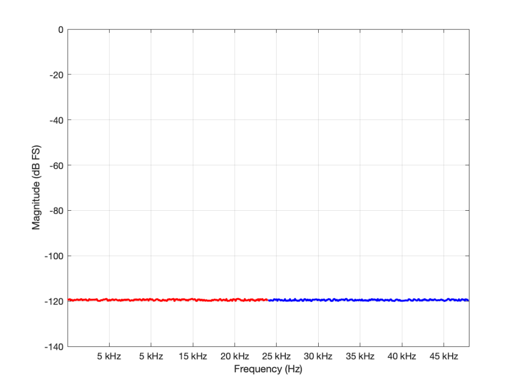
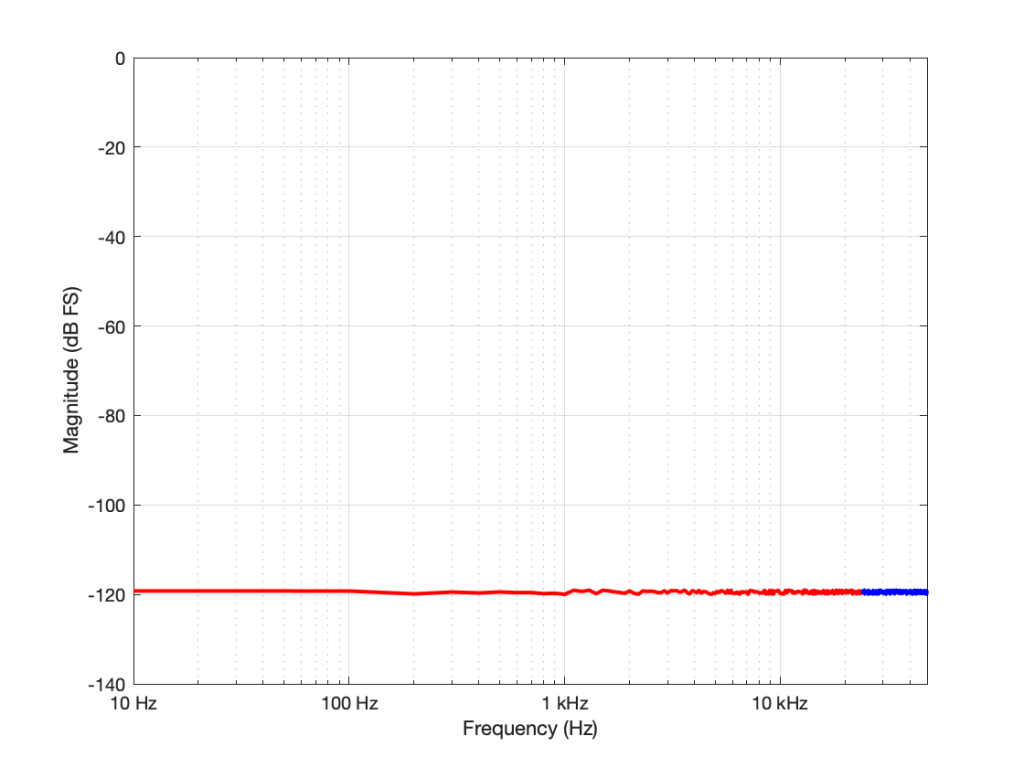
You may have looked at Figures 1 or 2 and are wondering why, if the noise floor is at -93 dB FS in a 16-bit system, I plotted it around -120 dB FS (give or take). The reason is related to the explanation I just gave above. I said in the captions that it’s from a 96 kHz system. This means that the noise extends to the Nyquist frequency at 48 kHz, and that total level is at -93 dB FS. We also know that, if I keep the noise the same, but half the bandwidth that I’m looking at, the level drops by 3 dB. Therefore I can either do math or I can make the following table:

Bandwidth of noise measurement in Hz	Level in dB FS
48,000	-93
24,000	-96
12,000	-99
6,000	-102
3,000	-105
1,500	-108
750	-111
375	-114
187.5	-117
93.75	-120

If you look carefully at the figures, you’ll see that there’s a point every 100 Hz. (It’s most easily visible in the low-frequency range of Figure 2.) So, the level of the noise that I see on a magnitude response plot like this is not only dependent on the noise level itself, but the bandwidths of the divisions that I’ve used to slice it up. In my case, the bandwidth per “slice” is about 100 Hz, so the noise level of each of those little contributors is at about -120 dB FS. If I had used slices only 50 Hz wide, it would show up at -123 instead…