Category: loudspeakers
Speakers and Sneakers
I recently received an email from someone asking the following question:
“I’ve been reading your blog for a while and a question popped up. What do you think of the practice of ”breaking in” speakers? Is there any truth to it or is it simply just another one of the million myths believed by audiophiles?”
To answer this question, I’ll tell a story.
At work, we have a small collection of loudspeakers – not only current B&O models, but older ones as well. In addition, of course, we have a number of loudspeakers made by our competitors. Many loudspeakers in this collection don’t get used very often, but occasionally, we’ll bring out a pair to have a listen as a refresher or reminder. Usually, the way this works is that one of us from the acoustics department will sneak into the listening room with a pair of loudspeakers, and set them up behind an acoustically transparent, but visually opaque curtain. The rest of us then get together and listen to the same collection of recordings at the same listening level, each of sitting in the same chair. We talk about how things sound, and then we open the curtain to see what we’ve been complaining about.
One day, about three years ago, it was my turn to bring in the loudspeakers, so I set up a pair of passive loudspeakers (not B&O) that have a reasonably good reputation. We had a listen and everyone agreed that the sound was less than optimal (to be polite…). No bass, harsh upper midrange, everything sounded like it was weirdly compressed. Not many of us had anything nice to say. I opened the curtain, and everyone in the room was surprised when they saw what we had listened to – since we would have all expected things to sound much better.
Later that day, I spoke with one of our colleagues who was not in the room, and I told him the story – no one liked the sound, but those speakers should sound better. His advice was to wait until next week, and play the same loudspeakers again – but the next time, play pink noise through them at a reasonably high level for a couple of hours before we listened. So, the next week, the day before we were scheduled to have our listening session, I set up the same speakers in the same locations in the room, and played pink noise at about 70 dB SPL through them overnight. The next morning, we had our blind listening session, and everyone in the room agreed that the sound was quite good – much better than what we heard last week. I opened the curtains and everyone was surprised again to see that nothing had changed. Or had it? I was as surprised as anyone, since my religious belief precludes this story from being true. But I was there… it actually happened.
So, what’s the explanation? Simple! Go to the store and buy two identical pairs of sneakers (or “running shoes” or “trainers”, depending on where you’re from). When you get home, take one pair out of the box, and wear them daily. After three or four months, take the pair that you left in the box and try them on. They will NOT feel the same as the pair you’ve been wearing. This is not a surprise – the leather and plastic and rubber in the sneakers you’ve been wearing has been stretched and flexed and now fits your foot better than the ones you have not been wearing. In addition, you’ll probably notice that the “old” ones are more flexible in the places where your foot bends, because you’ve been bending them.
It turns out (according to the colleague who suggested the pink noise trick who also used to design and make loudspeaker drivers for a living) that the suspension (the surround and spider) of a loudspeaker driver becomes more flexible by repeated flexing – just like your sneakers. If you take a pair of loudspeakers out of the box, plug them in, and start listening, they’ll be stiff. You need to work them a little to “loosen them up”.
This is not only true of new sneakers (and speakers) but also of sneakers (and speakers). For example, I keep my old sneakers around to use when I’m mowing the lawn. When I stick my foot into the sneakers that I haven’t worn all winter, they feel stiff, like a new pair, because they have not been flexed for a while. This is what happened to those speakers that I brought upstairs after sitting in the basement storage for years. The suspensions became stiff and needed to be moved a little before using them for listening to music.
A small problem that compounds the complexity of evaluating this issue is that we also “get used to” how things sound. So, as you’re “breaking in” a loudspeaker by listening to it, you are also learning and accommodating yourself to how it sounds, so you’re both changing simultaneously. Unless you have the option of playing a trick on people like I did with my colleagues, it’s difficult to make a reliable judgement of how big a difference this makes.
B&O Tech: Video Engine Customisation Part 1: Bass Management
#33 in a series of articles about the technology behind Bang & Olufsen loudspeakers
Earlier today (just after lunch), I had a colleague drop by to ask some technical questions about his new BeoVision 11. He’s done the setup with his external loudspeakers, but wanted to know if (mostly “how”…) he could customise his bass management settings to optimise his system. So, we went into the listening room to walk through the process. Since he was discussing this with some other colleagues around the lunch table, it turned out that we discovered that he wasn’t the only one who wanted to learn this stuff – so we wound up with a little group of 8 or 10 asking lots of questions that usually started with “but what if I wanted to…” After a half an hour or so, we all realised that this information should be shared with more people – so here I am, sharing.
This article is going to dive into the audio technical capabilities of what we call the “Video Engine” (the processing hardware inside the BeoPlay V1, the BeoVision 11, BeoVision Avant, and BeoSystem 4). For all of these devices, the software and its capabilities with respect to processing of audio signals are identical. Of course, the hardware capabilities are different – for example, the number of output channels are different from product to product – but everything I’m describing below can be done on all of those products.
One other warning: Almost of the menus that I direct you to in the text below are accessed as follows:
“MENU” button on remote control -> Setup -> Sound -> Speaker Group -> NAME -> Advanced Settings -> Bass Management
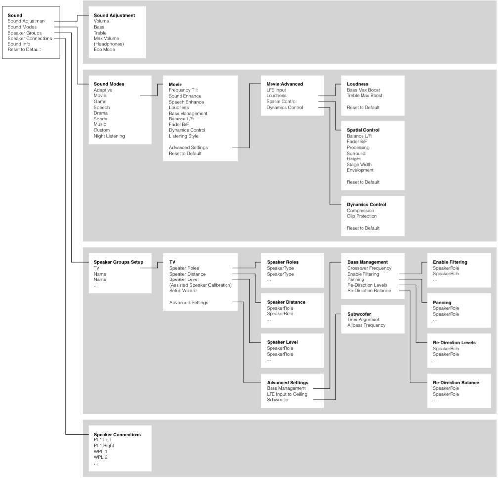
You can see this in the menu map, below.
So, let’s start by looking at a signal flow block diagram of the way the audio is processed inside the bass management processing.
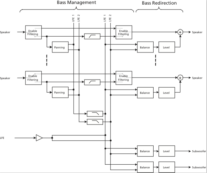
So, let’s start at the input to the system:
The “Speaker” signals coming in on the left are coming from the 16 output channels of the True Image upmixer (if you’re using it) or they are the direct 2.0, 5.1, or 7.1 (or other formats, if you’re weird like me) channels from the source. (We’ll ignore the LFE input for now – but we’ll come back to it later…)
The first thing the signals encounter is the switch labelled Enable Filtering (which is also the name of the menu item where you control this parameter). This where you decide whether you want the bass removed from the signal or not. For smaller loudspeakers (assuming that you have a big some in the same system) you will want to Enable the Filtering and remove the bass to re-direct it to the larger loudspeaker. If you have larger loudspeakers in the same system, you may not want to re-direct the signals. So, let’s say that you have BeoLab 20’s as the Left Front and Right Front (Lf / Rf for the rest of this article), BeoLab 17’s as the Left Surround and Right Surround (Ls / Rs), and the internal loudspeakers as the Centre Front (Cf), you will want to Enable Filtering on the Ls, Rs, and Cf signals. This will remove the bass from those channels and re-direct it somewhere else (to the 20’s – but we make that decision downstream…). You will not want to Enable Filtering for the 20’s since you’ll be using them as the “subwoofers”.
Assuming that you’ve enabled the filtering, then the signal takes the lower path and splits to go in two directions. The upper direction is to a high-pass filter. This is a 4th order highpass that is 6.02 dB down at the frequency chosen in the Crossover Frequency menu. We use a 4th order filter because the crossover in our bass management system is a 4th order Linkwitz-Riley design. As you can see in the block diagram, the output of the highs filter is routed directly to the output to the loudspeaker. The low path in the split goes to a block called Panning. This is where you decide, on a channel-by-channel basis, whether the signal should be routed to the left or the right bass channel (or some mix of the two). For example, if you have a Ls loudspeaker that you’re bass managing, you will probably want to direct its bass to the Left bass channel. The Rs loudspeaker’s bass will probably direct to the Right bass channel, and the Cf loudspeaker’s bass will go to both. (Of course, if, at the end of all this, you only have one subwoofer, then it doesn’t matter, since the Left and Right bass channels will be summed anyway.) The outputs of all the panning blocks are added together to form the two bass channels – although, you may notice in the block diagram, they are still full-range signals at this point (internally) in the signal flow, since we haven’t low-pass filtered them yet.
Next, the “outputs” of the two bass channels are low-pass filtered using a 4th order filter on each. Again, this is due to the 4th order Linkwitz-Riley crossover design. The cutoff frequency of these two low pass filters are identical to the highpass filters which are all identical to each other. There is a very good reason for this. Whenever you apply a minimum-phase filter (which ours are, in this case) of any kind to an audio signal, you get two results: one is a change in the magnitude response of the signal, the other is a change in its phase response. One of the “beautiful” aspects of the Linkwitz-Riley crossover design is that the Low Pass and High Pass filters are 360° out-of-phase with each other at all frequencies. This is (sort of…) the same as being in-phase at all frequencies – so the signals add back together nicely. If, however, you use a different cutoff frequency for the low and high pass components, then the phase responses don’t line up nicely – and things don’t add back together equally at all frequencies. If you have audio channels that have the same signals (say, for example, the bass guitar in both the Lf and Rf at the same time – completely correlated) then this also means that you’ll have to use the same filter characteristics on both of those channels. So, the moral of the story here is that, in a bass management system, there can be only one crossover frequency to rule them all.
You may be wondering why we add the signals before we apply the low-pass filter. The only reason for this was an optimisation of the computing power – whether we apply the filter on each input channel (remember, there are up to 16 of those…) or on two summed outputs, the result is the same. So, it’s smarter from a DSP MIPS-load point of view to use two filters instead of 16 if the result is identical (all of our processing is in floating point, so there’s no worry of overloading the system internally).
Now comes the point where we take the low-frequency components of the bass-managed signals and add them to the incoming LFE channel. You may notice a little triangle on that LFE channel before it gets summed. This is not the +10 dB that is normally added to the LFE channel – that has already happened before it arrived at the bass management system. This gain is a reduction, since we’re splitting the signal to two internal bass channels that may get added back together (if you have only one subwoofer, for example). If we didn’t drop the gain here, you’d wind up with too much LFE in the summed output later.
Now we have the combined LFE and bass management low-frequencies on two (left and right) bass channels, ready to go somewhere – but the question is “where?” We have two decisions left to make. The first is the Re-direction Balance. This is basically the same as a good-old-fashioned “balance” control on your parents’ stereo system. Here you can decide (for a given loudspeaker output) whether it gets the Left bass channel, the Right bass channel, or a combination of the two (you only have three options here). If you have a single subwoofer, you’ll probably be smart to take the “combination” option. If you have separate Left and Right subwoofers, then you’ll want to direct the Left bass channel to the left subwoofer and the right to the right.
Finally, you get to the Bass Re-direction Level menu. This is where you decide the gain that should be applied to the bass channel that is sent to the particular loudspeaker. If you have one subwoofer and you want to send it everything, then its Redirection level will by 0 dB and the other loudspeakers will be -100 dB. If you want to send bass everywhere, then set everything to 0 dB (this is not necessarily a good idea – unless you REALLY like bass…).
It’s important to note that ANY loudspeaker connected in your system can be treated like a “subwoofer” – which does not necessarily mean that it has a “subwoofer” Speaker Role. For example, in my system, I use my Lf and Rf loudspeakers as the Lf and Rf channels in addition to the subwoofers. This can be seen in the menus as the Lf and Rf Re-direction levels set to 0 dB (and all others are set to -100 dB to keep the bass out of the smaller loudspeakers).
Special Treatment for Subwoofers
As you can see in the block diagram, there are two “subwoofer” outputs which, as far as the bass management is concerned, are identical to other loudspeakers. However, the Subwoofer outputs have two additional controls downstream for customising the alignment with the rest of the system. The first is a Time Alignment adjustment which can be set from -30 ms to +30 ms. If this value is positive, then the subwoofer output is delayed relative to the rest of the system. If it’s negative, then the rest of the system is delayed relative to the subwoofer. There are lots of reasons why you might want to do either of these on top of your Speaker Distance adjustment – but I’m not going to get into that here.
The second control is a first-order Allpass filter. This will be 90° out of phase at the frequency specified on the screen – going to 180° out at a maximum in the high frequencies. The reason to use this would be to align for phase response differences between your subwoofer’s high end and your main “main loudspeakers'” low-end. Say, for example, you have a closed-box subwoofer, but ported (or slave driver-based) main loudspeakers. You may need some phase correction in a case like this to clean up the addition of the signals across the crossover region. Of course, if you have different main loudspeakers, then one allpass filter on your subwoofer can’t correct for all of the different responses in one shot. Of course, if you don’t want to have an allpass filter in your subwoofer signal path, you can bypass it.
For more information about the stuff I talked about here (including cool things like phase response plots of the allpass filter), check out the Technical Sound Guide for the Video Engine-based products. This is downloadable from this page for example.
B&O Tech: The Naked Truth V
#32 in a series of articles about the technology behind Bang & Olufsen loudspeakers
This posting: something new, something old…
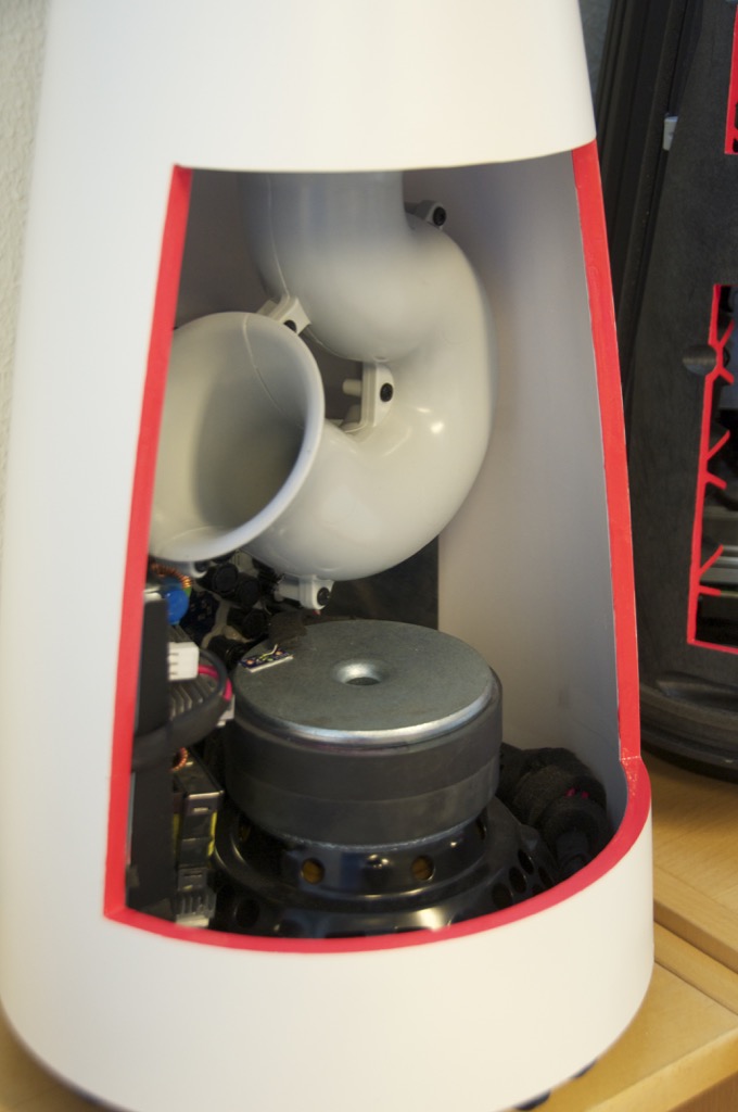
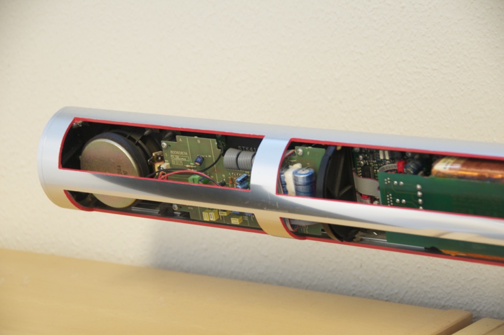
First, the insides of the BeoLab 14 subwoofer. The obvious part is the port curling around to get the right length in a somewhat shorter package. This concept has been around for a while as you can see when you look at a trumpet or a tuba…
The silver-coloured disc right below the bottom of the port is the pole piece of the woofer. The black ring around this is the ferrite magnet. In the background you can see the circuit boards containing the power supply, DSP and amplifiers for the sub and the satellites. For a better view of this, check out this page.
The reasons the end of the port is flared like a trumpet bell is to reduce the velocity of the air at the end of the pipe. This reduces turbulence which, in turn, means that there is less noise or “port chuffing” at the resonant frequency of the port. Of course, the other end of the port at the top of the subwoofer is also flared for the same reason.
As I mentioned in a previous posting, the DSP is constantly calculating the air velocity inside the port and doesn’t allow it to exceed a value that we determined in the tuning. This doesn’t mean that it’s impossible to hear the turbulence – if you test the system with a sine tone, you’ll hear it – but that was a tuning decision we made. This is because we pushed the output to a point that is almost always inaudible with music – but can be heard with sine tones. If we hadn’t done that, the cost would have been a subwoofer with less bass output.


Now for something a little older… This is a BeoLab 3500 (we’re not looking at the BeoLab 7-4 on the shelf below)
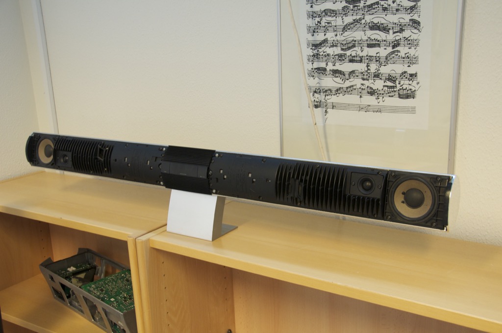
Below is a close-up of the tweeter and woofer. You may notice that you can see light through the edge of the surround of the woofer. This is because we cut it with a knife for a different demonstration – it’s not normal… You can also see the fins which help to keep the electronics cool.


As you can see in the photos below, all the electronics are inside the woofer enclosures. The tweeter has its own built-in chamber, so it’s sealed from the woofer enclosure.


B&O Tech: Naked Truth IV
#29 in a series of articles about the technology behind Bang & Olufsen loudspeakers
Sorry – I’ve been busy lately, so I haven’t been too active on the blog.
Here are some internal shots of the BeoLab 17 and BeoLab 20 loudspeakers. As you can see in the shot of the back of the BeoLab 17, the entire case is the enclosure is for the woofer. The tweeter has its own enclosure which seals it from the woofer cabinet.


What’s not obvious in the photos of the BeoLab 20 is that the midrange and woofer cabinets are separate sealed boxes. There is a bulkhead that separates the two enclosures cutting across the loudspeaker just below the midrange driver.


Cymatics v2
Cymatics v1
B&O Tech: How B&O Makes a Loudspeaker – Part 2/2
#31 in a series of articles about the technology behind Bang & Olufsen loudspeakers
from www.recordere.dk when they visited Struer for the BeoLab 20 launch.
B&O Tech: Near… Far…
#27 in a series of articles about the technology behind Bang & Olufsen loudspeakers
Introduction
To begin with, please watch the following video.
One thing to notice is how they made Grover sound near and far. Two things change in his voice (yes, yes, I know. It’s not ACTUALLY Grover’s voice. It’s really Yoda’s). The first change is the level – but if you’re focus on only that you’ll notice that it doesn’t really change so much. Grover is a little louder when he’s near than when he’s far. However, there’s another change that’s more important – the level of the reverberation relative to the level of the “dry” voice (what recording engineers sometimes call the “wet/dry mix”). When Grover is near, the sound is quite “dry” – there’s very little reverberation. When Grover is far, you hear much more of the room (more likely actually a spring or a plate reverb unit, given that this was made in the 1970’s).
This is a trick that has been used by recording engineers for decades. You can simulate distance in a mix by adding reverb to the sound. For example, listen to the drums and horns in the studio version of Penguins by Lyle Lovett. Then listen to the live version of the same people playing the same tune. Of course, there are lots of things (other than reverb) that are different between these two recordings – but it’s a good start for a comparison. As another example, compare this recording to this recording. Of course, these are different recordings of different people singing different songs – but the thing to listen for is the wet/dry mix and the perception of distance in the mix. Another example is this recording compared to this recording.
So, why does this trick work? The answer lies inside your brain – so we’ll have to look there first.
Distance Perception in the Mix
If you’re in a room with your eyes closed, and someone in the room starts talking to you, you’ll be pretty good at estimating where they are in the room – both in terms of angular location (you can point at them) and distance. This is true, even if you’ve never been in the room before. Very generally speaking, what’s going on here is that your brain is automatically comparing:
- the two sounds coming into your two ears – the difference between these two signals tells you a lot about which direction the sound is coming from, AND
- the direct sound from the source to the reflected sound coming from the room. This comparison gives you lots of information about a sound source’s distance and the size and acoustical characteristics of the room itself.
If we do the same thing in an anechoic chamber (a room where there are no echoes, because the walls absorb all sound) you will still be good at estimating the angle to the sound source (because you still have two ears), but you will fail miserably at the distance estimation (because there are no reflections to help you figure this out).
If you want to try this in real life, go outside (away from any big walls), close your eyes, and try to focus on how far away the sound sources appear to be. You have to work a little to force yourself to ignore the fact that you know where they really are – but when you do, you’ll find that things sound much closer than they are. This is because outdoors is relatively anechoic. If you go to the middle of a frozen lake that’s covered in fluffy snow, you’ll come as close as you’ll probably get to an anechoic environment in real life. (unless you do this as a hobby)
So, the moral of the story here is that, if you’re doing a recording and you want to make things sound far away, add reflections and reverberation – or at least make them louder and the direct sound quieter.
Distance Perception in the Listening Room
Let’s go back to that example of the studio recording of Lyle Lovett recording of Penguins. If you sit in your listening room and play that recording out of a pair of loudspeakers, how far away do the drums and horns sound relative to you? Now we’re not talking about whether one sounds further away than the other within the mix. I’m asking, “If you close your eyes and try to guess how far away the snare drum is from your listening position – what would you guess?”
For many people, the answer will be approximately as far away as the loudspeakers. So, if your loudspeakers are 3 m from the listening position, the horns (in that recording) will sound about 3 m away as well. However, this is not necessarily the case. Remember that the perception of distance is dependent on the relative levels of the direct and reflected sounds at your ears. So, if you listen to that recording in an anechoic chamber, the horns will sound closer than the loudspeakers (because there are no reflections to tell you how far away things are). The more reflective the room’s surfaces, the more the horns will sound further away (but probably no further than the loudspeakers, since the recording is quite dry).
This effect can also be the result of the width of the loudspeaker’s directivity. For example, a loudspeaker that emits a very narrow beam (like a laser, assuming that were possible) would not send any sound towards the walls – only towards the listening position. So, this would have the same effect as having no reflection (because there is no sound going towards the sidewalls to reflect). In other words, the wider the dispersion of the sound from the loudspeaker (in a reflective room) the greater the apparent distance to the sound (but no greater than the distance to the loudspeakers, assuming that the recording is “dry”).
Loudspeaker directivity
So, we’ve established that the apparent distance to a phantom image in a recording is, in part, and in some (perhaps most) cases, dependent on the loudspeaker’s directivity. So, let’s concentrate on that for a bit.
Let’s build a very simple loudspeaker. It’s a model that has been used to simulate the behaviour of a real loudspeaker, so I don’t feel too bad about over-simplifying too much here. We’ll build an infinite wall with a piston in it that moves in and out. For example:
Here, you can see the piston (in red) moving in and out of the wall (in grey) with the resulting sound waves (the expanding curves) moving outwards in the air (in white).
The problem with this video is that it’s a little too simple. We also have to consider how the sound radiation off the front of the piston will be different at different frequencies. Without getting into the physics of “why” (if you’re interested in that, you can look here or here or here for an explanation) a piston has a general behaviour with repeat to the radiation patten of the sound wave it generates. Generally, the higher the frequency, the narrower the “beam” of sound. At low frequencies, there is basically no beam – the sound is emitted in all directions equally. At high frequencies, the beam to be very narrow.
The question then is “how high a frequency is ‘high’?” The answer to that lies in the diameter of the piston (or the diameter of the loudspeaker driver, if we’re interested in real life). For example, take a look at Figure 1, below.

Figure 1 shows how loud a signal will be if you measure it at different directions relative to the face of a piston that is 10″ (25.4 cm) in diameter. Two frequencies are shown – 100 Hz (the blue curve) and 1.5 kHz (the green curve). Both curves have been normalised to be the same level (100 dB SPL – although the actual value really doesn’t matter) on axis (at 0°). As you can see in the plot, as you move off to the side (either to 90° or 270°) the blue curve stays at 100 dB SPL. So, no matter what your angle relative to on-axis to the woofer, 100 Hz will be the same level (assuming that you maintain your distance). However, look at the green curve in comparison. As you move off to the side, the 1.5 kHz tone drops by more than 20 dB. Remember that this also means that (if the loudspeaker is pointing at you and the sidewall is to the side of the loudspeaker) then 100 Hz and 1.5 kHz will both get to you at the same level. However, the reflection off the wall will have 20 dB more level at 100 Hz than at 1.5 kHz. This also means, generally, that there is more energy in the room at 100 Hz than there is at 1.5 kHz because, if you consider the entire radiation of the loudspeaker averaged over all directions at the same time the lower frequency is louder in more places.
This, in turn, means that, if all you have is a 10″ woofer and you play music, you’ll notice that the high frequency content sounds closer to you in the room than the low frequency content.
If the loudspeaker driver is smaller, the effect is the same, the only difference is that the effect happens at a higher frequency. For example, Figure 2, below shows the off-axis response for two frequencies emitted by a 1″ (2.54 cm) diameter piston (i.e. a tweeter).

Notice that the effect is identical, however, now, 1.5 kHz is the “low frequency region for the small piston, so it radiates in all directions equally (seen as the blue curve). The high frequency (now 15 kHz) becomes lower and lower in level as you move off to the side of the driver, going as low as -20 dB at 90°.
So, again, if you’re listening to music through that tweeter, you’ll notice that the frequency content at 1.5 kHz sounds further away from the listening position than the content at 15 kHz. Again, the higher the frequency, the closer the image.
Same information, shown differently
If you trust me, figures 1 and 2, above, show you that the sound radiating off the front of a loudspeaker driver gets narrower with increasing frequency. If you don’t trust me (and you shouldn’t – I’m very untrustworthy…) then you’ll be saying “but you only showed me the behaviour at two frequencies… what about the others?” Well, let’s plot the same basic info differently, so that we can see more data.
Figure 3, below, shows the same 10″ woofer, although now showing all frequencies from 20 Hz to 20 kHz, and all angles from -90° to +90°. However, now, instead of showing all levels (in dB) we’re only showing 3 values, at -1 dB, -3 dB, and -10 dB. ( These plots are a little tougher to read until you get used to them. However, if you’re used to looking at topographical maps, these are the same.)

Now you can see that, as you get higher in frequency, the angles where you are within 1 dB of the on-axis response gets narrower, starting at about 400 Hz. This means that a 10″ diameter piston (which we are pretending to be a woofer) is “omnidirectional” up to 400 Hz, and then gets increasingly more directional as you go up.
Figure 4 shows the same information for a 1″ diameter piston. Now you can see that the driver is omnidirectional up to about 4 kHz. (This is not a coincidence – the frequency is 10 times that of the woofer because the diameter is one tenth.)
Normally, however, you do not make a loudspeaker out of either a woofer or a tweeter – you put them together to cover the entire frequency range. So, let’s look at a plot of that behaviour. I’ve put together our two pistons using a 4th-order Linkwitz-Riley crossover at 1.5 kHz. I have also not included any weirdness caused by the separation of the drivers in space. This is theoretical world where the tweeter and the woofer are in the same place – an impossible coaxial loudspeaker.

In Figure 5 you can see the effects of the woofer’s directivity starting to beam below the crossover, and then the tweeter takes over and spreads the radiation wide again before it also narrows.
So what?
Why should you care about understanding the plot in Figure 5? Well, remember that the narrower the radiation of a loudspeaker, the closer the sound will appear to be to you. This means that, for the imaginary loudspeaker shown in Figure 5, if you’re playing a recording without additional reverberation, the low frequency stuff will sound far away (the same distance as the loudspeakers), So will a narrow band between 3 kHz and 4 kHz (where the tweeter pulls the radiation wider). However, the materials in the band around 700 Hz – 2 kHz and in the band above 7 kHz will sound much closer to you.
Another way to express this is to show a graph of the resulting level of the reverberant energy in the listening room relative to the direct sound, an example of which is shown in Figure 6. (This is a plot copied from “Acoustics and Psychoacoustics” by David Howard and Jamie Angus).

This shows a slightly different loudspeaker with a crossover just under 3 kHz. This is easy to see in the plot, since it’s where the tweeter starts putting more sound into the room, thus increasing the amount of reverberant energy.
What does all of this mean? Well, if we simplify a little, it means that things like voices will pull apart in terms of apparent distance. Consonant sounds like “s” and “t” will appear to be closer than vowels like “ooh”.
So, whaddya gonna do about it?
All of this is why one of the really important concerns of the acoustical engineers at Bang & Olufsen is the directivity of the loudspeakers. In a previous posting, I mentioned this a little – but then it was with regards to identifying issues related to diffraction. In that case, directivity is more of a method of identifying a basic problem. In this posting, however, I’m talking about a fundamental goal in the acoustical design of the loudspeaker.
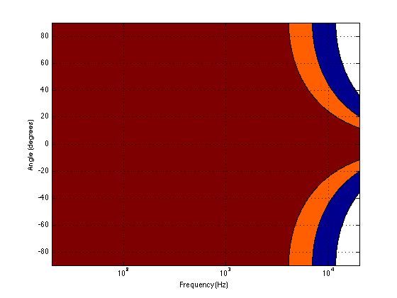
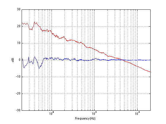
For example, take a look at Figures 7 and 8 and compare them to Figure 9. It’s important to note here that these three plots show the directivities of three different loudspeakers with respect to their on-axis response. The way this is done is to measure the on-axis magnitude response, and call that the reference. Then you measure the magnitude response at a different angle, and then calculate the difference between that and the reference. In essence, you’re pretending that the on-axis response is flat. This is not to be interpreted that the three loudspeakers shown here have the same on-axis response. They don’t. Each is normalised to its own on-axis response. So we’re only considering how the loudspeaker compares to itself.

Figure 7, above, shows the directivity behaviour of a commercially-available 3-way loudspeaker (not from Bang & Olufsen). You can see that the woofer is increasingly beaming (the directivity gets narrow) up to the 3 – 5 kHz area. The midrange is beaming up above 10 kHz or so. So, a full band signal will sound distant in the low end, in the 6-7 kHz range and around 15 kHz. By comparison, signals at 2-4 kHz and 10-15 kHz will sound quite close.

Figure 8, above, shows the directivity behaviour of a 3-way loudspeaker we made as a rough prototype. This is just a woofer, midrange and tweeter, each in its own MDF box – nothing fancy – except that the tweeter box is not as wide as the midrange box which is narrower than the woofer box. You can see that the woofer is beaming (the directivity gets narrow) just above 1 kHz – although it has a very weird wide directivity at around 650 Hz for some reason. The midrange is beaming up from 5kHz to 10 kHz, and then the tweeter gets wide. So, this loudspeaker will have the same problem as the commercial loudspeaker
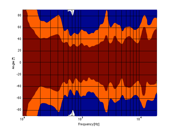
As you can see, the loudspeaker with the directivity shown in Figure 9 (the BeoLab 5) is much more constant as you change frequency (in other words, the lines are more parallel). It’s not perfect, but it’s a lot better than the other two – assuming that constant directivity is your goal. You can also see that the level of the signal that is within 1 dB of the on-axis response is quite wide compared with the loudspeakers in Figures 7 and 8. The loudspeaker in Figure 7 not only beams in the high frequencies, but also has some strange “lobes” where things are louder off-axis than they are on-axis (the red lines).
When you read B&O’s marketing materials about the reason why we use Acoustic Lenses in our loudspeakers, the main message is that it’s designed to spread the sound – especially the high frequencies – wider than a normal tweeter, so that everyone on the sofa can hear the high hat. This is true. However, if you ask one of the acoustical engineers who worked on the project, they’ll tell you that the real reason is to maintain constant directivity as well as possible in order to ensure that the direct-to-reverberant ratio in your listening room does not vary with frequency. However, that’s a difficult concept to explain in 1 or 2 sentences, so you won’t hear it mentioned often. However, if you read this paper (which was published just after the release of the BeoLab 5), for example, you’ll see that it was part of the original thinking behind the engineers on the project.
Addendum 1.
I’ve been thinking more about this since I wrote it. One thing that I realised that I should add was to draw a comparison to timbre. When you listen to music on your loudspeakers in your living room, in a best-case scenario, you hear the same timbral balance that the recording engineer and the mastering engineer heard when they worked on the recording. In theory, you should not hear more bass or less midrange or more treble than they heard. The directivity of the loudspeaker has a similar influence – but on the spatial performance of the loudspeakers instead of the timbral performance. You want a loudspeaker that doesn’t alter the relative apparent distances to sources in the mix – just like you don’t want the loudspeakers to alter the timbre by delivering too much high frequency content.
Addendum 2.
One more thing… I made the plot below to help simplify the connection between directivity and Grover. Hope this helps.

Audio Mythinformation: 16 vs 24 bit recordings
Preface: Lincoln was right
There is a thing called “argument from authority” which is what happens when you trust someone to be right about something because (s)he knows a lot about the general topic. This is used frequently by pop-documentaries on TV when “experts” are interviewed about something. Example: “we asked an expert in underwater archeology how this piece of metal could wind up on the bottom of the ocean, covered in mud and he said ‘I don’t know’ so it must have been put there by aliens millions of years ago.” Okay, I’m exaggerating a little here, but my point is that, just because someone knows something about something, doesn’t mean that (s)he knows everything about it, and will always give the correct answers for every question on the topic.
In other words, as Abraham Lincoln once said: “Don’t believe everything you read on the Internet.”
Of course, that also means that also applies to everything that follows in the posting below (arrogantly assuming that I can be considered to be an authority on anything), so you might as well stop reading and go do something useful.
My Inspiration
There has been some discussion circulating around the Interweb lately about the question of whether the “new” trend to buy “high-resolution” audio files with word lengths of 24 bits actually provides an improvement in quality over an audio file with “only” 16 bits.
One side of this “religious” war comes from the people who are selling the high-res audio files and players. The assumed claim is that 24 bits makes a noticeable improvement in audio quality (over a “mere” 16 bits) that justifies asking you to buy the track again – and probably at a higher price.
The other side of the war are bloggers and youtube enthusiasts who write things like (a now-removed) article called “24/192 Music Downloads… and why they make no sense” (which, if you looked at the URL, is really an anti-Pono rant) and “Bit Depth & The 24 Bit Audio Myth“
Personally, I’m not a fan of religious wars, so I’d like to have a go at wading into the waters in a probably-vain attempt to clear up some of the confusion and animosity that may be caused by following religious leaders.
Some background
If you don’t know anything about how an audio signal is converted from analogue to digital, you should probably stop reading here and go check out this page or another page that explains the same thing in a different way.
Now to recap what you already know:
- An analogue to digital converter makes a measurement of the instantaneous voltage of the audio signal and outputs that measurement as a binary number on each “sample”
- The resolution of that converter is dependent on the length of the binary number it outputs. The longer the number, the higher the resolution.
- The length of a binary number is expressed in Binary digITs or BITS.
- The higher the resolution, the lower the noise floor of the digital signal.
- In order to convert the artefacts caused by quantisation error from distortion to program-dependent noise, dither is used. (Note that this is incorrectly called “quantisation noise” by some people)
- In a system that uses TPDF (Triangular Probability Distribution Function) dither, the noise has a white spectrum, meaning that is has equal energy per Hz.
A good rule of thumb in a PCM system with TPDF dithering is that the dynamic range of the system is approximately 6 * the number of bits – 3 dB. For example, the dynamic range of a 16-bit system is 6*16-3 = 93 dB. Some people will say that this is the signal-to-noise ratio of the system, however, this is only correct if your signal is always as loud as it can be.
Let’s think about what, exactly, we’re saying here. When we measure the dynamic range of a system, we’re trying to find out what the difference is (in dB) between (1) the loudest sound you can put through the system without clipping and (2) the noise floor of the system.
The goal of an engineer when making a piece of audio gear (or of a recording engineer when making a recording) is to make the signal (the music) so loud that you can’t hear the noise – but not so loud that the signal clips and therefore distorts. There are three ways to improve this: you can either (1) make your gear capable of making the signal louder, (2) design your gear so that it has less noise, or (3) both of those things. In either case, what you are trying to maximise is the ratio of the signal to the noise. In other words, relative to the noise level, you want the signal as high as possible.
However, this is a rather simplistic view of the world that has two fatal flaws:
The first problem is that (unless you like most of the music my kids like) the signal itself has a dynamic range – it gets loud and it also gets quiet. This can happen over long stretches of time (say, if you’re listening to a choral piece written by Arvo Pärt) or over relatively short periods of time (say, the difference between the sharp peak of a rim shot on a snare and the decay of a piano noise in the middle of the piece of music I’ve plotted below.)
You should note that this isn’t a piece that I use to demonstrate wide dynamic range or anything – I just started looking through my classical music collection for a piece that can demonstrate that music has loud AND quiet sections – and this was the second piece I opened (it’s by the Ahn Trio – I was going alphabetically…) So don’t make a comment about how I searched for an exceptional example of the once recording in the history of all recordings that has dynamic range. That would be silly. If I wanted to do that, I would have dug out an Arvo Pärt piece – but Arvo comes after Ahn in the alphabet, so I didn’t get that far.

The portion of this piece that I’ve highlighted in Figure 1 (the gray section in the middle) has a peak at about 1 dB below full scale, and, at the end gets down to about -46 dB below that. (You might note that there is a higher peak earlier in the piece – but we don’t need to worry about that.) So, that little portion of the music has a dynamic range of about 45 dB or so – if we’re just dumbly looking at the plot.
So, this means that we want to have a recording system and a playback system for this piece of music that has can handle a signal as loud as that peak without distorting it – but has a constant noise floor that is quiet enough that I won’t hear it at the end of that piano note decaying at the end of that little section I’ve highlighted.
What we’re really talking about here is more accurately called the dynamic range of the system (and the recording). We’re only temporarily interested in the Signal to Noise ratio, since the actual signal (the music) has a constantly varying level. What’s more useful is to talk about the dynamic range – the difference (in dB) between the constant noise of the system (or the recording) and the maximum peak it can produce. However, we’ll come back to that later.
The second problem is that the noise floor caused by TPDF dither is white noise, which means that you have equal energy per Hertz as we’ve seen before. We can also reasonably safely assume that the signal is music which usually consists of a subset of all frequencies at any moment in time (if it had all frequencies present, it would sound like noise of some colour instead of Beethoven or Bieber), that are probably weighted like pink noise – with less and less energy in the high frequencies.
In a worst-case situation, you have one note being played by one instrument and you’re hoping that that one note is going to mask (or “drown out”) the noise of the system that is spread across a very wide frequency range.
For example, let’s look again at the decay of that piano note in the example in Figure 1. That’s one note on a piano, dropping down to about -40-something dB FS, with a small collection of frequencies (the fundamental frequency of the pitch and its multiples), and you’re hoping that this “signal” is going to be able to mask white noise that stretches in frequency band from something below 20 Hz all the way up past 20 kHz. This is worrisome, at best.
In other words, it would be easy for a signal to mask a noise if the signal and the noise had the same bandwidth. However, if the signal has a very small bandwidth and the noise has a very wide bandwidth, then it is almost impossible for the signal to mask the noise.
In other words, the end of the decay of one note on a piano is not going to be able to cover up hiss at 5 kHz because there is no content at 5 kHz from the piano note to do the covering up.
So, what this means is that you want a system (either a recording or a piece of audio gear) where, if you set the volume such that the peak level is as loud as you want it to be, the noise floor of the recording and the playback system is inaudible at the listening position. (We’ll come back to this point at the end.) This is because the hope that the signal will mask the noise is just that – hope. Unless you listen to “music” that has no dynamic range and is constantly an extremely wide bandwidth, then I’m afraid that you may be disappointed.
One more thing…
There is another assumption that gets us into trouble here – and that is the one I implied earlier which says that all of my audio gear has a flat magnitude response. (I implied it by saying that we can assume that the noise that we get is white.)
Let’s look at the magnitude response of a pair of earbud headphones that millions and millions of people own. I borrowed this plot from this site – but I’m not telling you which earbuds they are – but I will say that they’re white. It’s the top plot in Figure 2.

This magnitude response is a “weighting” that is applied to everything that gets into the listener’s ears (assuming that you trust the measurement itself). As you can see if you put in a signal that consists of a 20 Hz tone and a 200 Hz tone that are equal in level, then you’ll hear the 200 Hz tone about 40 dB louder than the 20 Hz tone. Remember that this is what happens not only to the signal you’re listening to, but also the noise of the system and the recording – and it has an effect.
For example, if we measure a 16-bit linear PCM digital system with TPDF dithering, we’ll see that it has a 93.3 dB dynamic range. This means that the RMS level of a sine wave (or another signal) that is just below clipping the system (so it’s as loud as you can get before you start distorting) is 93.3 dB louder than the white noise noise floor (yes, the repetition is intentional – read it again). However, that is the dynamic range if the system has a magnitude response that is +/- 0 dB from 0 Hz to half the sampling rate.
If, however, you measured the dynamic range through those headphones I’m talking about in Figure 2, then things change. This is because the magnitude response of the headphones has an effect on both the signal and the noise. For example, if the signal you used to measure the maximum capabilities of the system were a 3 kHz sine tone, then the dynamic range of the system would improve to about 99 dB. (I measured this using the filter I made to “fake” the magnitude response – it’s shown in the bottom of Figure 2.)
Remember that, with a flat magnitude response, the dynamic range of the 16-bit system is about 93 dB. By filtering everything with a weird filter, however, that dynamic range changes to 99 dB IF THE SIGNAL WE USE TO MEASURE THE SYSTEM IS a 3 kHz SINE TONE.
The problem now is that the dynamic range of the system is dependent on the spectrum of the signal we use to measure the peak level with – which will also be true when we consider the signal to noise ratio of the same system. Since the spectrum of the music AND the dither noise are both filtered by something that isn’t flat, the SNR of the system is dependent on the frequency content of the music and how that relates to the magnitude response of the system.
For example, if we measured the dynamic range of the system shown above using sine tones at different frequencies as our measurement signal, we would get the values shown in Figure 3

If you’re looking not-very-carefully-at-all at the curve in Figure 3, you’ll probably notice that it’s basically the curve on the bottom of Figure 2, upside down. This makes sense, since, generally, the filter will attenuate the total power of the noise floor, and the signal used to make the dynamic range measurement is a sine wave whose level is dependent on the magnitude response. What this means is that, if your system is “weak” at one frequency band, then the signal to noise ratio of the system when the signal consists of energy in the “weak” band will be worse than in other bands.
Another way to state this is: if you own a pair of those white earbuds, and you listen to music that only has bass in it (say, the opening of this tune) you might have to turn up the level so much to hear the bass that you’ll hear the noise floor in the high end.
Wrapping up
As I said at the beginning, some people say “more bits are better, so you should buy all your music again with 24-bit versions of your 16-bit collection”. Some other people say “24-bits is a silly waste of money for everyone”.
What’s the truth? Probably neither of these. Let’s take a couple of examples to show that everyone’s wrong.
Case 1: You listen to music with dynamic range and you have a good pair of loudspeakers that can deliver a reasonably high peak SPL level. You turn up the volume so that the peak reaches, say, 110 dB SPL (this is loud for a peak, but if it only happens now and again, it’s not that scary). If your recording is a 16-bit recording, then the noise floor is 93 dB below that, so you have a wide-band noise floor of 17 dB SPL which is easily audible in a quiet room. This is true even when the acoustic noise floor of the room is something like 30 dB SPL or so, since the dither noise from the loudspeaker has a white noise characteristic, whereas acoustic background noise in “real life” is usually pink in spectrum. So, you might indeed hear the high-frequency hiss. (Note that this is even more true if you have a playback system with active loudspeakers that protect themselves from high peaks – they’ll reduce the levels of the peaks, potentially causing you to push up the volume knob even more, which brings the noise floor up with it.)
Case 2: You have a system with a less-than-flat magnitude response (i.e. a bass roll-off) and you are listening to music that only has content in that frequency range (i.e. the bass), so you turn up the volume to hear it. You could easily hear the high-frequency noise content in the dither if that high frequency is emphasised by the playback system.
Case 3: You’re listening to your tunes that have no dynamic range (because you like that kind of music) over leaky headphones while you’re at the grocery store shopping for eggs. In this case, the noise floor of the system will very likely be completely inaudible due to the making by the “music” and the background noise of announcements of this week’s specials.
The Answer
So, hopefully I’ve shown that there is no answer to this question. At least, there is no one-size-fits-all answer. For some people, in some situations, 16 bits are not enough. There are other situations where 16 bits is plenty. The weird thing that I hope that I’ve demonstrated is that the people who MIGHT benefit from higher resolution are not necessarily those with the best gear. In fact, in some cases, it’s people with worse gear that benefit the most…
… but Abraham Lincoln was definitely right. Stick with that piece of advice and you’ll be fine.
Appendix 1: Noise shaping
One of the arguments against 24-bit recordings is that a noise-shaped 16-bit recording is just as good in the midrange. This is true, but there are times when noise shaping causes playback equipment some headaches, since it tends to push a lot of energy up into the high frequency band where we might be able to hear it (at least that’s the theory). The problem is that the audio gear is still trying to play that “signal”, so if you have a system that has issues, for example, with Intermodulation Distortion (IMD) with high-frequency content (like a cheap tweeter, as only one example) then that high-frequency noise may cause signals to “fold down” into audible bands within the playback gear. So noise shaping isn’t everything it’s cracked up to be in some cases.