In Part 2 of this series, I wrote the following sentence:
The easiest (and possibly best) way to do this is to create white noise with a triangular probability distribution function and a peak-to-peak amplitude of ± 1 quantisation level.
That’s a very busy sentence, so let’s unpack it a little.
Rolling the dice
If you roll one die, you have an equal probability of rolling any number between 1 and 6 (inclusive). Let’s roll one die 100 times counting the number of times we get a 1, or a 2, or a 3, and so on up to 6.
| Number rolled | Number of times the number was rolled | Percentage of times the number was rolled |
| 1 | 17 | 17 |
| 2 | 14 | 14 |
| 3 | 15 | 15 |
| 4 | 15 | 15 |
| 5 | 21 | 21 |
| 6 | 18 | 18 |
(Note that the percentage of times each number was rolled is the same as the number of times each number was rolled only because I rolled the die 100 times.)
If I plot those results, it looks like Figure 1.
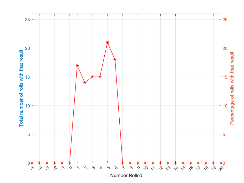
It may be weird, but I’ve plotted the number of times I rolled -5 or 13 (for example). These are 0 times because it’s impossible to get those numbers by rolling one die. But the reason I put those results in there will make more sense later.
Let’s keep rolling the die. If I do it 1,000,000 times instead of 100, I get these results:
| ed | Number of times the number was rolled | Percentage of times the number was rolled |
| 1 | 166225 | 16.6225 |
| 2 | 166400 | 16.6400 |
| 3 | 166930 | 16.6930 |
| 4 | 167055 | 16.7055 |
| 5 | 166501 | 16.6501 |
| 6 | 166889 | 16.6889 |
Now, since I rolled many, many, more times, it’s more obvious that the six results have an equal probability. The more I roll the die, the more those numbers get closer and closer to each other.
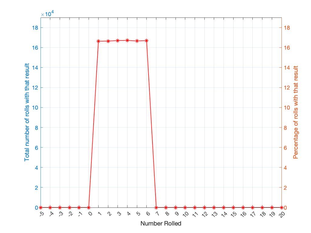
Take a look at the shape of the plot above. The area under the line from 1 to 6 (inclusive) is almost a rectangle because the six numbers are all almost the same.
The shape of that plot shows us the probability of rolling the six numbers on the die, so we call it a probability density function or PDF. In this case, we see a rectangular PDF.
But what happens if we roll two dice instead? Now things get a little more complicated, since there is more than one way to get a total result, as shown in the table below.
| Total | ||||||
| 2 | 1+1 | |||||
| 3 | 1+2 | 2+1 | ||||
| 4 | 1+3 | 2+2 | 3+1 | |||
| 5 | 1+4 | 2+3 | 3+2 | 4+1 | ||
| 6 | 1+5 | 2+4 | 3+3 | 4+2 | 5+1 | |
| 7 | 1+6 | 2+5 | 3+4 | 4+3 | 5+2 | 6+1 |
| 8 | 2+6 | 3+5 | 4+4 | 5+3 | 6+2 | |
| 9 | 3+6 | 4+5 | 5+4 | 6+3 | ||
| 10 | 4+6 | 5+5 | 6+4 | |||
| 11 | 5+6 | 6+5 | ||||
| 12 | 6+6 |
As can be (hopefully) seen in the table, there is only one way to roll a 2, and there’s only one way to roll a 12. But there are 6 different ways to roll a 7. Therefore, if you’re rolling two dice, it’s 6 times more likely that you’ll roll a 7 than a 12, for example.
If I were to roll two dice 1,000,000 times, I would get a PDF like the one shown in Figure 3.
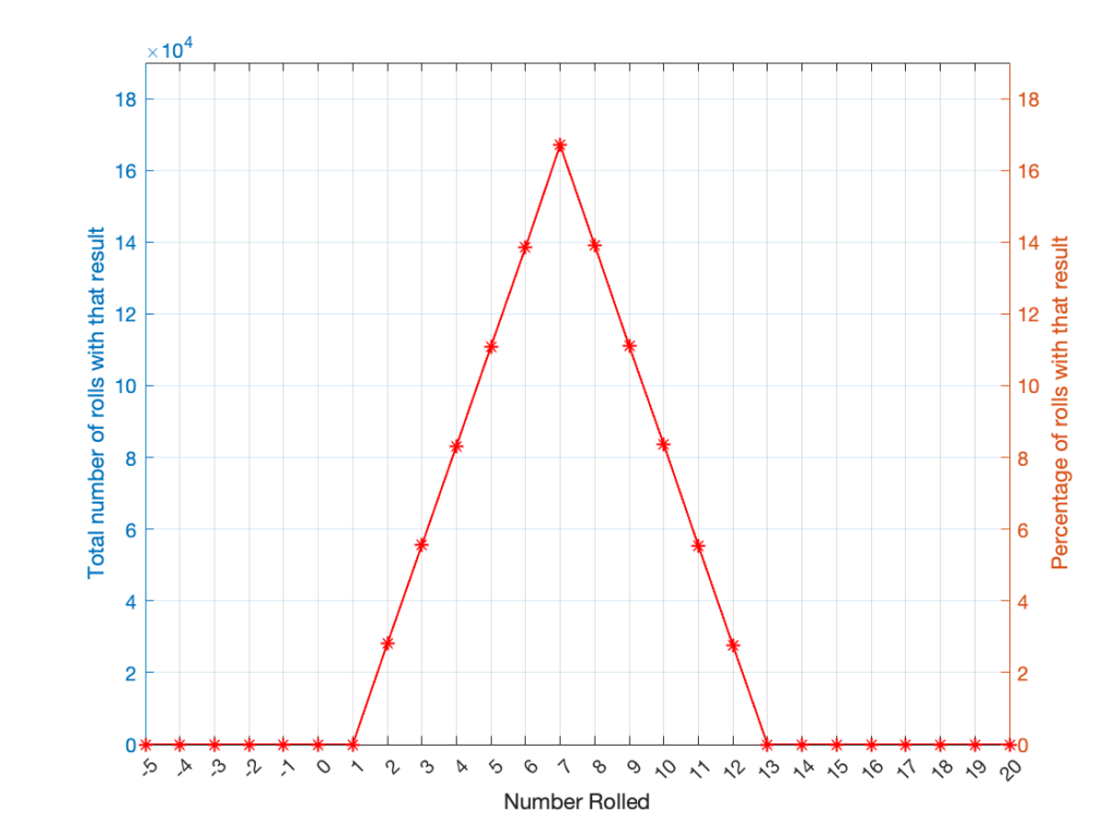
I won’t explain why this would be considered to be a triangular PDF.
Whether you roll one die or two dice, the number you get is random. In other words, you can’t use the past results to predict what the next number will be. However, if you are rolling one die, and you bet that you’ll roll a 6 every time, you’ll be right about 16.7% of the time. If you’re rolling two dice and you bet that you’ll roll a 12 every time, you’ll only be right about 2.8% of the time.
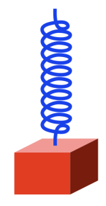
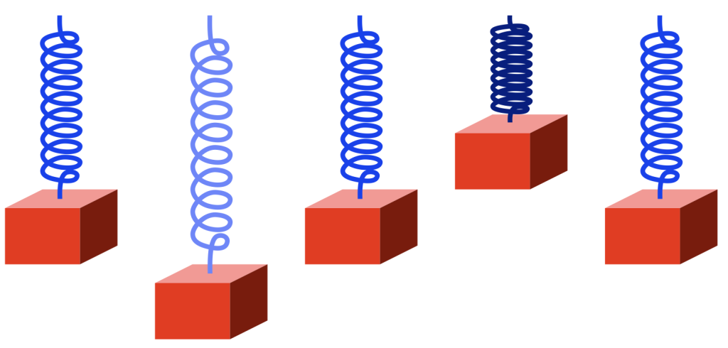
Let’s take two dice of different colours, say, one red die and one blue die. We’ll roll both dice again, but instead of adding the two values, we’ll subtract the blue value from the red one. If we do this 1,000,000 times, we’ll get something like the results shown below in Figure 4.
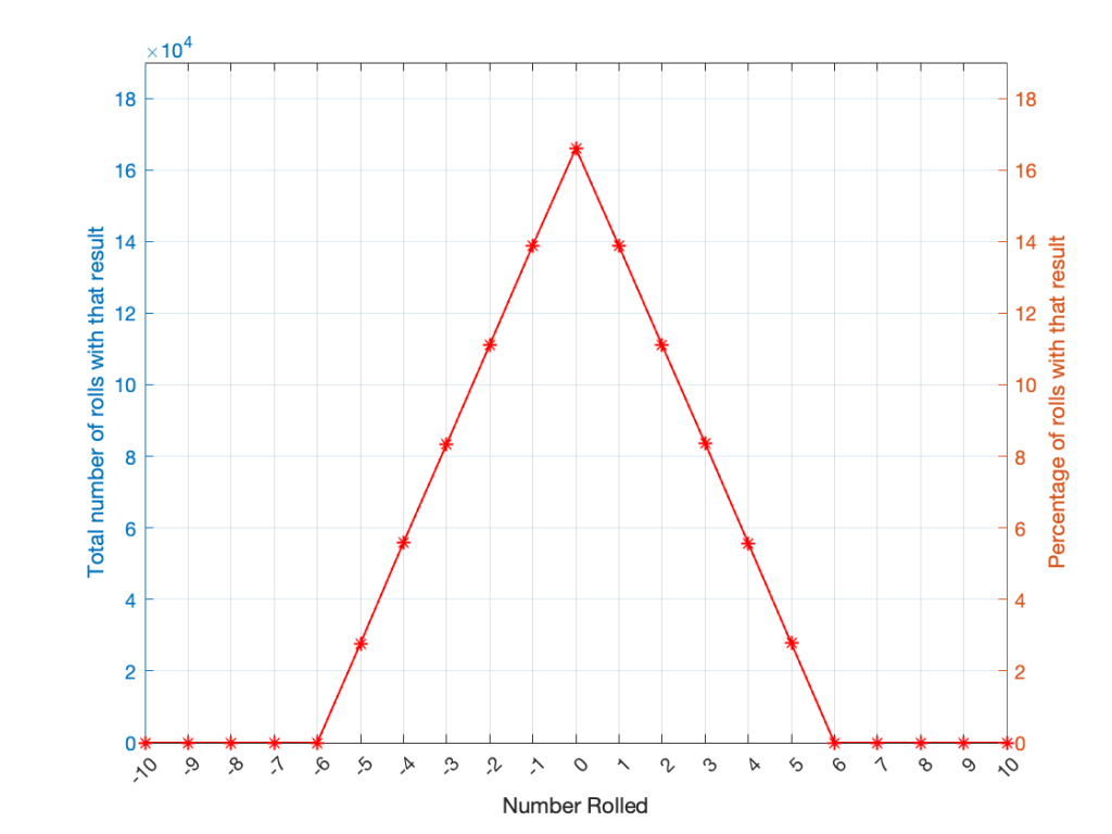
Notice that the probability density function keeps the same shape, it’s just moved down to a range of ±5 instead of 2 to 12.
Generating noise
In audio, noise is a sound that is completely random. In other words, just like the example with the dice, in a digital audio signal, you can’t predict what the next sample value will be based on the past sample values. However, there are many different ways of generating that random number and manipulating its characteristics.
Let’s start with a computer algorithm that can generate a random number between 0 and 1 (inclusive) with a rectangular PDF. We’ll then ask the algorithm to spit out 1,000,000 values. If the numbers really are random, and the computer has infinite precision, then we’ll probably get 1,000,000 different numbers. However, we’re not really interested in the numbers themselves – we’re interested in how they’re distributed between 0.00 and 1.00. Let’s say we divide up that range into 100 steps (or “buckets”) that are 0.01 wide and count how many of our random numbers fall into each group. So, we’ll count how many are between 0.0 and 0.01, between 0.01 and 0.02, and so on up to 0.99 to 1.00. We’ll get something like Figure 5.
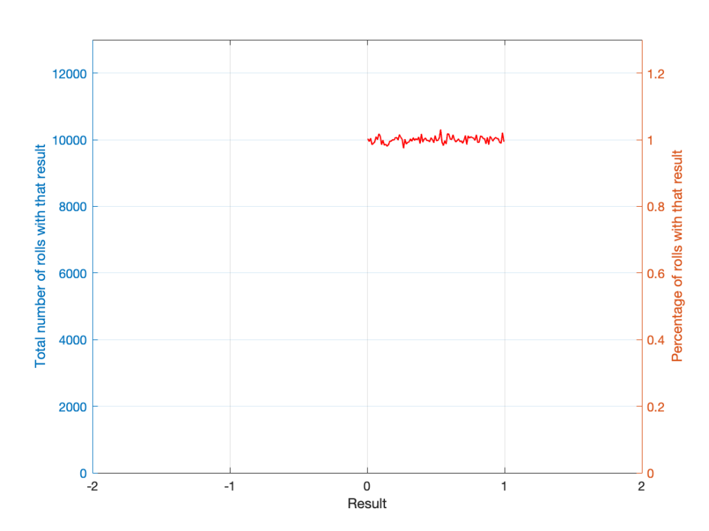
I’ve only plotted the probabilities of the possible values: 0 to 1, which winds up showing only the top of the rectangle in the rectangular PDF.
If I generate 1,000,000 random numbers with that algorithm, and then subtract 1,000,000 other random numbers, one by one, and find the probabilities of the result, the answer will be familiar.
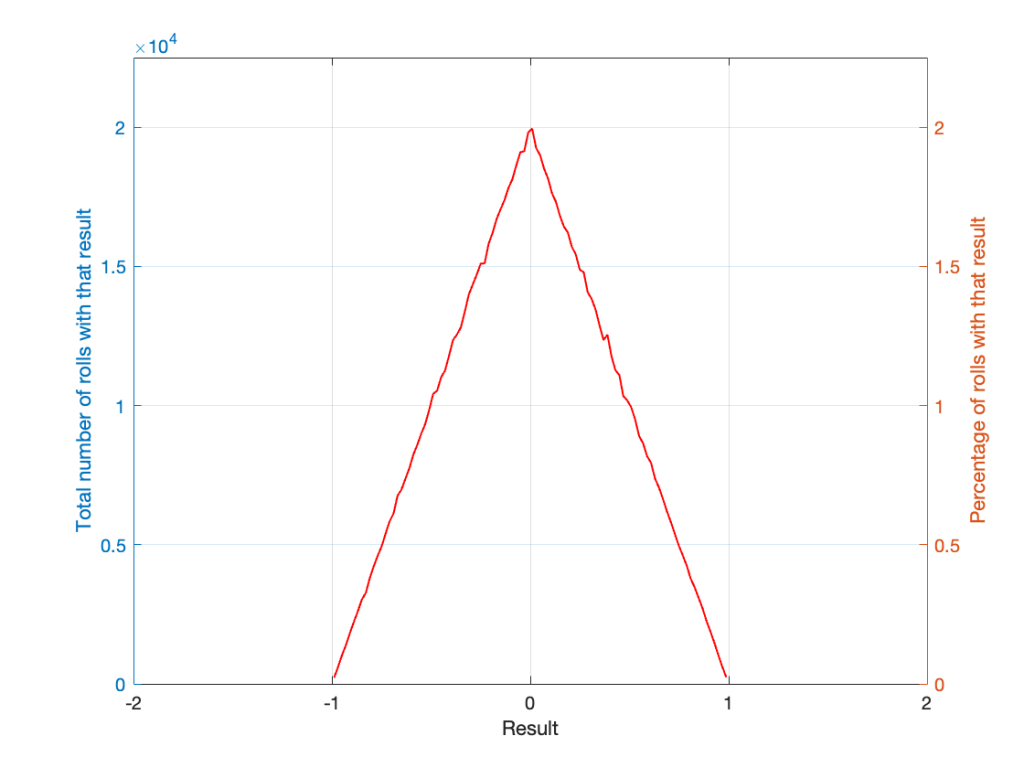
So, this is how we make the noise that’s added to the signal. If, for each sample, you generate two random numbers (making sure that your algorithm has a rectangular PDF) and subtract one from the other, you have the dither signal that will have a maximum level of ±1 quantisation level.
- The signal (with a maximum range of ±1) is scaled up by multiplying it by 2(NumberOfBits-1)-2
- then you add the result of the dither generator
- then the total is rounded to the nearest integer value
- and then the result is scaled back down by a factor of 2(NumberOfBits-1) to bring its back down to a range of ±1 to get it ready for exporting to a standard audio file format like .wav or .flac.
In other words, assuming that you have an audio signal called “Signal” that has a range of ±1 and consists of floating point values:
ScaleUp = 2^(Bitdepth-1)-2
ScaleDown = 2^(Bitdepth-1)

TpdfDither = rand(LengthOfSignal) - rand(LengthOfSignal)

QuantisedDitheredSignal = round(Signal * ScaleUp + TpdfDither) / ScaleDown;