Links to:
DFT’s Part 1: Some introductory basics
DFT’s Part 2: It’s a little complex…
DFT’s Part 3: The Math
DFT’s Part 4: The Artefacts
DFT’s Part 5: Windowing
In Part 5, we talked about the idea of using a windowing function to “clean up” a DFT of a signal, and the cost of doing so. We talked about how the magnitude response that is given by the DFT is rarely “the Truth” – and that the amount that it’s not True is dependent on the interaction between the frequency content of the signal, the signal envelope, the windowing function, the size of the FFT, and the sampling rate. The only real solution to this problem is to know what-not-to-believe when you look at a DFT output.
However, we “only” looked at the artefacts on the magnitude response in the previous posting. In this last posting, we’ll dig a little deeper and NOT throw away the phase information. The problem is that, when you’re windowing, you’re not just looking at a screwed up version of the magnitude response, you’re also looking at a screwed up phase response as well.
We saw in Part 1 and Part 2 how the phase of a sinusoidal waveform can be converted to the sum of a real and an imaginary component. (In other words, if you add a cosine and a sine of the same frequency with very specific separate gains applied to them, the result will be a sinusoidal waveform with any amplitude and phase that you want.) For this posting, we’ll be looking at the artefacts of the same windowing functions that we’ve been working on – but keeping the real and imaginary components separate.
Rectangular windowing
We’ll start by looking at a plot from the previous post, which I’ve duplicated below.
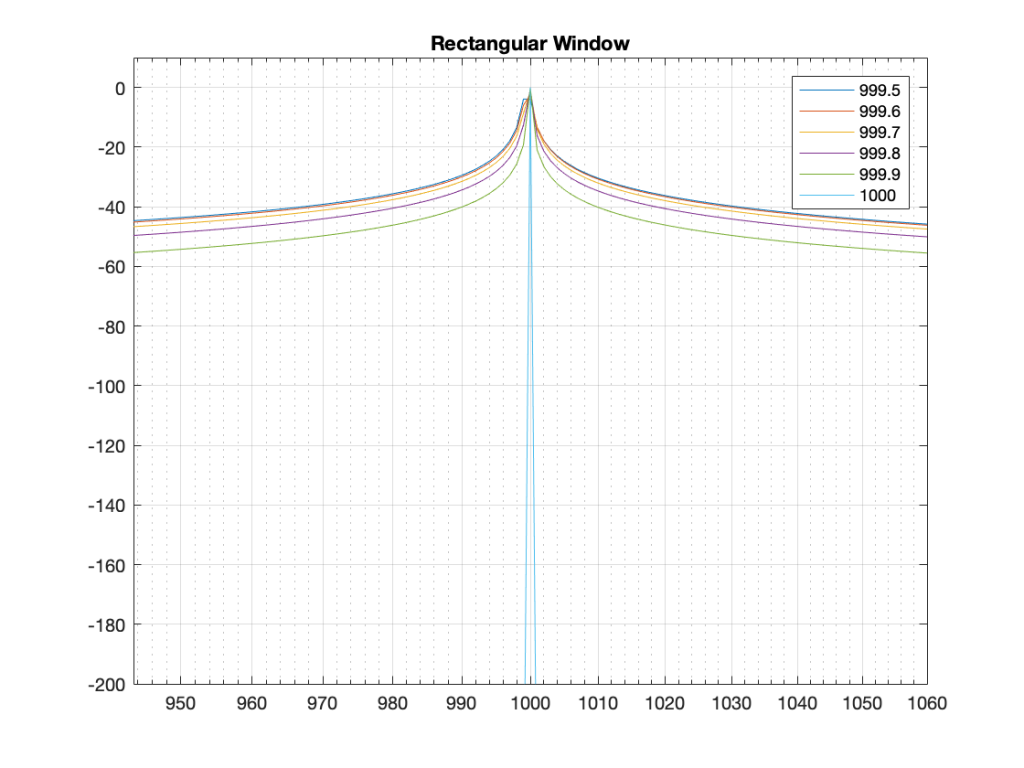
The way I did the plot in Figure 1 was to create a sine wave with a given frequency, do a DFT of that, and plot the magnitude of the result. I did that for 6 different frequencies, ranging from 1000 Hz (exactly on a bin centre frequency) to 999.5 Hz (halfway to the adjacent bin centre frequency).
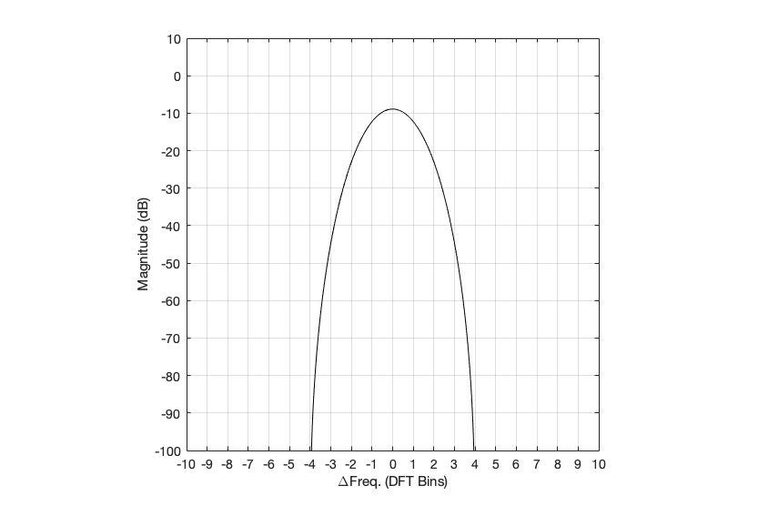
There’s a different way to plot this, which is to show the result of the DFT output, bin by bin, for a sinusoidal waveform with a frequency relative to the bin centre frequency. This is shown below in Figure 2.
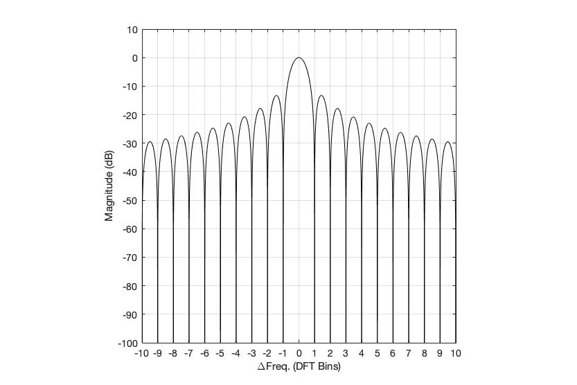
The relationship between the frequency of the signal, the frequency centres of the DFT bin, and the resulting magnitude in dB. Note that the X-axis is frequency, measured in distance between bin frequencies or “bin widths”.
Now we have to talk about how to read that plot… This tells me the following (as examples):
- If the bin centre frequency EXACTLY matches the frequency of the signal (therefore, the ∆ Freq. = 0) then the magnitude of that bin will be 0 dB (in other words, it will give me the correct answer).
- If the bin centre frequency is EXACTLY an integer number of bin widths away from the frequency of the signal (therefore, the ∆ Freq. = … -10, -9, – 8… -3, -2, -1, 1, 2, 3, … 8, 9, 10, …) then the magnitude of that bin will be -∞ dB (in other words, it will have no output).
- These two first points are why the light blue curve is so good in Figure 1.
- If the frequency of the signal is half-way between two bins (therefore, the ∆ Freq. = -0.5 or +0.5), then you get an output of about -4 dB (which is what we also saw in the blue curve in Figure 25 in Part 5.
- If the frequency of the signal is an integer number away from half-way between two bins (for example, ∆ Freq. = -2.5, -1.5, 1.5, or 2.5, etc… ) then the output of that bin will be the value shown at the tops of those bumps in the plots… (For example, if you mark a dot at each place where ∆ Freq. = ±x.5 on that curve above, and you join the dots, you’ll get the same curve as the curve for 999.5 Hz in Figure 1.)
So, Figure 2 shows us that, unless the signal frequency is exactly the same as the bin centre frequency, then the DFT’s magnitude will be too low, and there will be an output from all bins.
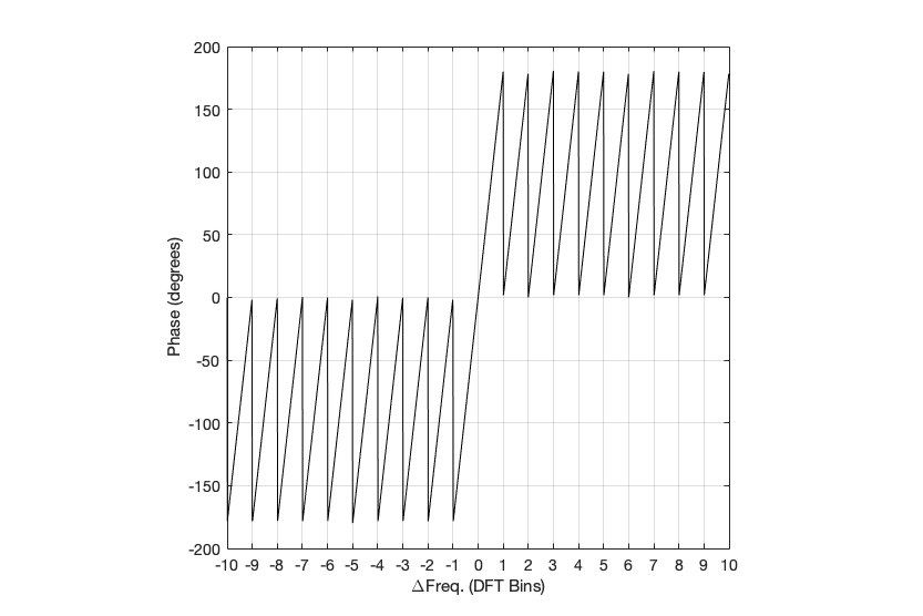
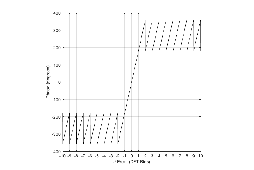
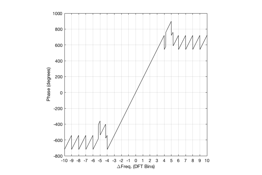
The relationship between the frequency of the signal, the frequency centres of the DFT bin, and the resulting phase in degrees.
Figure 3 shows us the same kind of analysis, but for the phase information instead. The important thing when reading this plot is to keep the magnitude response plot in mind as well. For example:
- when the bin frequency matches the signal frequency (∆ Freq. = 0) then the phase error is 0º.
- When the signal frequency is an integer number of bin widths away from the bin frequency, then it appears that the phase error is either 0º or ±180º, but neither of these is true, since the output is -∞ dB – there is no output (remember the magnitude response plot).
- There is a gradually increasing error from 0º to ±180º (depending on whether you’re going up or down in frequency)( as the signal frequency moves from being adjacent to one bin or the next.
- When you signal frequency crosses the bin frequency, you get a polarity flip (the vertical lines in the sawtooth shape in the plot).
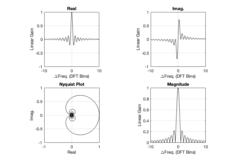
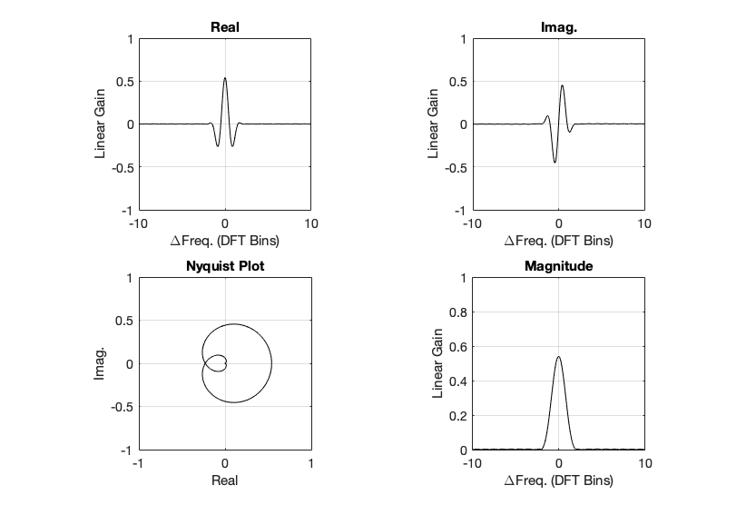
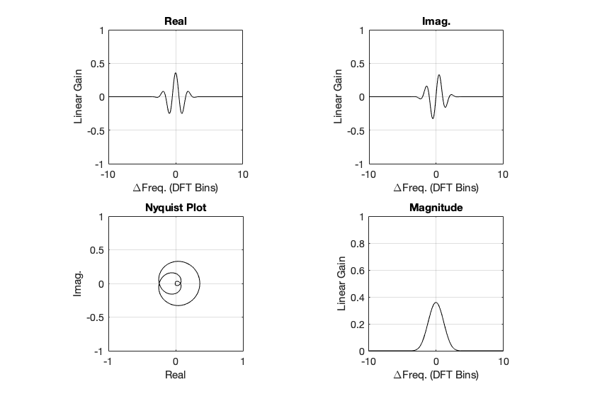
The top two plots show the same relationship as in Figures 2 and 3, but divided into the various components, as explained below.
Figure 4, above, shows the same information, plotted differently.
- The bottom right plot shows the magnitude response (exactly the same as shown in Figure 2) on a linear scale instead of in dB.
- The top two plots show the Real and Imaginary components, which, combined, were used to generate the Magnitude and Phase plots. (Remember from Parts 1 and 2 that the Real component is like looking at the response from above, and the Imaginary component is like looking at the response from the side.)
- The Nyquist plot is difficult, if not impossible to understand if you’ve never seen one before. But looking at the entire length of the animation in Figure 5, below, should help. I won’t bother explaining it more than to say that it (like the Real vs. Freq. and the Imaginary vs. Freq. plots) is just showing two dimensions of a three-dimensional plot – which is why it makes no sense on its own without some prior knowledge.
The Real, Imaginary, and Nyquist plots from Figure 4, viewed from different angles.
Hopefully, I’ve said enough about the plots above that you are now equipped to look at the same analyses of the other windowing functions and draw your own conclusions. I’ll just make the occasional comment here and there to highlight something…
Hann Window

Generally, the things to note with the Hann window are the wider centre lobe, but the lower side lobes (as compared to the rectangular windowing function).


Hamming window

The interesting thing about the Hamming window is that the lobes adjacent to the main lobe in the middle are lower. This might be useful if you’re trying to ignore some frequency content next to your signal’s frequency.


Blackman Window

The Blackman window has a wider centre lobe, but the side lobes are lower in level.


Blackman Harris window
Although the Blackman-Harris window results in a wider centre lobe, as you can see in Figure 18, the side lobes are all at least 90 dB down from that…
Wrapping up
I know that there’s lots left out of this series on DFT’s. There are other windowing functions that I didn’t talk about. I didn’t look at the math that is used to generate the functions… and I just glossed over lots of things. However, my intention here was not to do a complete analysis – it was a just an introductory discussion to help instil a lack of trust – or a healthy suspicion about the results of a DFT (or FFT – depending on how fast you do the math….).
Also, a reason I did this series was as a set-up, so when I write about some other topics in the future (like the actual resolution of 16-bit LPCM audio in a fixed point world, or the implications of making a volume control in the digital domain as just two examples…), I can refer back to this, pointing out what you can and cannot believe is the plots that I haven’t even made yet…