This is the start of what will be a series of posts that are an attempt to answer a question about the pro’s and con’s of implementing a volume control in the digital domain. When I first thought about how to answer this question, I thought I could do it in a couple of sentences – but the more I thought about it, the more I realised that the answer is complicated…
There’s no doubt in my mind that I’m making this answer more complicated than necessary, but, as Carl Sagan once said, “If you wish to make apple pie from scratch, you must first create the universe.”
So, to begin, we have to define what “noise” is from the point of view of audio engineering.
On the one hand, we can define it simply. “Noise” is a random signal. We can be more accurate and say that this means that the amplitude of a noise signal cannot be predicted using a knowledge of what has come before in time.
If I flip a coin, it will be either heads or tails. I can’t predict this. It will be random. If I flip it 100 times, and, by some strange coincidence, I get 100 “tails”, there is still a 50% chance of getting a tails on the 101st flip. What has happened before can, in no way, be used to predict what is about to happen.
Of course, what is about to happen on the 101st flip has a limited number of possible outcomes. I cannot flip the coin and get “dog” as a result… (this sounds silly, but it will come in handy later…) Just like I cannot roll two dice and get a 13…
In LPCM digital audio, a noise signal is one where each individual sample in the signal has a random value that is in no way related to any of the previous samples. Its range (the set of possible values from which we can pick our random number) may be limited (depending on the specific characteristics of the noise signal and what may have come before), but it will be random.
Typically, when you are talking to someone in audio about noise, they describe it using a colour as the first descriptor. So, you’ll hear of “white noise” and “pink noise”, as the two most popular examples. For the purposes of this series of postings, we’ll only be talking about white noise. So, what is this?
One definition that you’ll see thrown around a lot says something like “white noise is a random signal that has equal energy per linear bandwidth” or “… equal energy per hertz” or “…equal intensity at different frequencies” or something like this. These descriptions are sort of true if you don’t want to get into temporal details, which, unfortunately, is exactly where we’re headed…
The good thing about those definitions is that they describe a general characteristic of white noise. If you take a white noise signal, and you measure the intensity of (or the energy in) the signal for a given bandwidth (say, a bandwidth of 100 Hz ranging from 200 Hz to 300 Hz) then it will be the same in another frequency range with the same bandwidth (say, a bandwidth of 100 Hz ranging from 1,000 Hz to 1,100 Hz). Note that these two bandwidths are the same in hertz – not in a multiplier like octaves or semitones or decades. So, if you have white noise that has a total bandwidth of 0 Hz to 20,000 Hz, then you will have the same amount of energy in the 0 – to – 10,000 Hz band as you will in the 10,000 – to – 20,000 Hz band. In other words (to us humans), there is as much energy in the top octave of the signal as in the rest of the bandwidth combined.
This is why white noise sounds like “bright” and “hissy” (similar to the “ss” sound in “hissy”) and not “darker” like the “sh” sound in “ash” (as they incorrectly claim here…). Since white is a “bright” colour, then we use the word “white” to describe the frequency-dependent energy distribution of “white” noise.
However, this is not really true. The truth is that a white noise signal has an equal probability per bandwidth of having the same energy level. This little detail is usually left out, partly because it’s complicated, and partly because it doesn’t matter in most cases in the real world. However, in our case, it does.
Let’s look at an example. I made a white noise signal in Matlab using the statement
rand(SignalLength, 1) – rand(SignalLength, 1)
where SignalLength is the length of the noise signal in samples, and the 1 means that I’m doing this for 1 audio channel…. mono is so retro…
You may be wondering why I did a
rand() – rand()
instead of just a
rand().
the simple answer for now was that I wanted to make the signal “balanced” on either side of the zero line and the rand() function in Matlab has a range of 0 to 1.I know… I could have done this by saying
2 * (rand(SignalLength, 1) – 0.5)
but there is another reason that we’ll get into later…)
I then used a DFT to find the magnitude response of this signal. The result – both the signal and its magnitude response – are shown below in Figure 1.
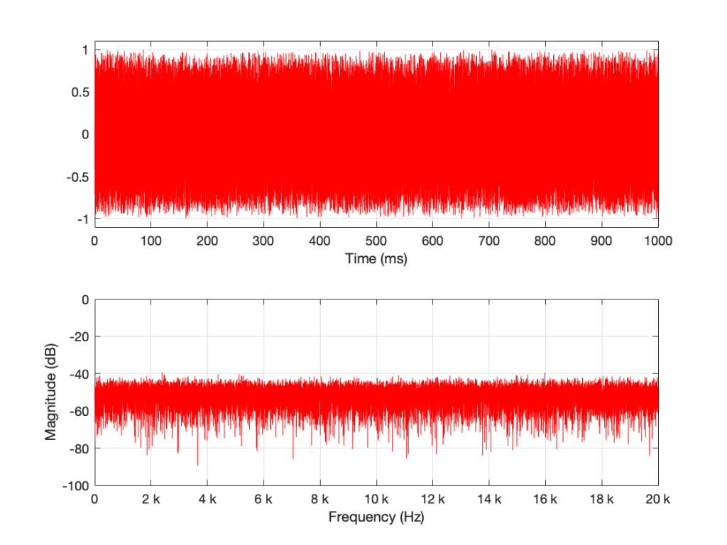
Some additional information that is really not important: The sampling rate of this signal is 2^16 (65,536 Hz), and I did a 2^16 point DFT, so I have one frequency bin per hertz. (If this last bit of information is confusing, but interesting, please start reading this…)
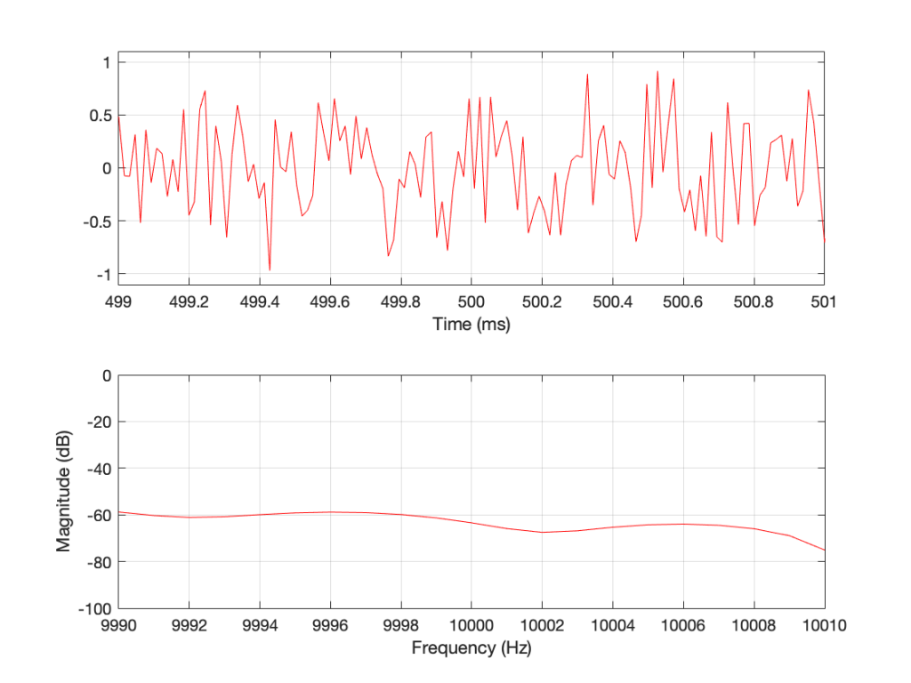
You may notice that the magnitude is “flat” – meaning that it generally doesn’t slope upwards or downwards. However, you will also notice that it is certainly not “flat” – meaning that it is not a perfectly straight line. In fact, if we zoom in on both plots, we can see Figure 2.
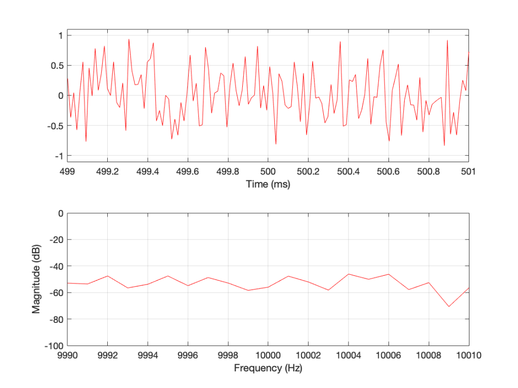
Notice that we do NOT have an equal amount of energy per hertz… if we did, then the bottom plot would be a flat line.
If I do all of that again – make a new noise sample the same way (with a new set of random numbers) and plot the result, and a zoomed in version, I get Figures 3 and 4.
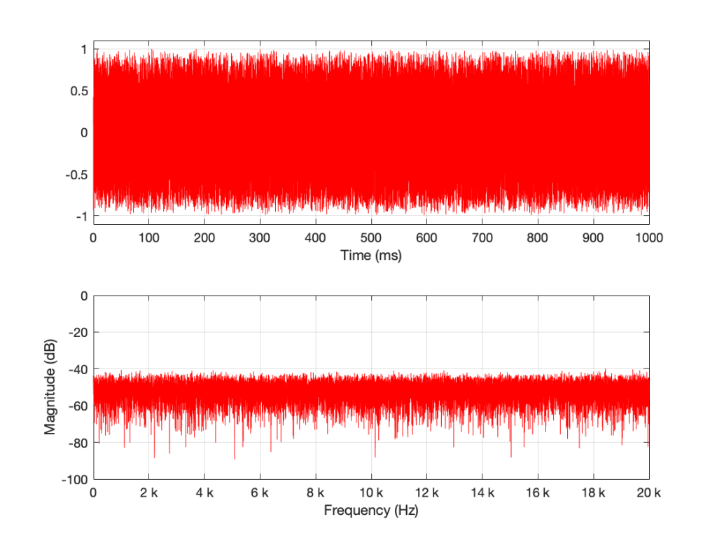
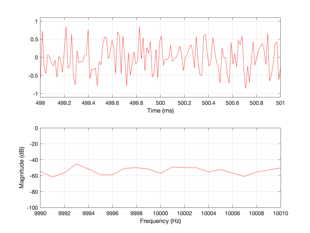
Compare Figures 1 and 3 or Figure 2 and 4. You’ll notice that they have similar characteristics overall – but not only are they NOT identical, they are completely different (on a sample-by-sample or a DFT bin-by-bin comparison).
Let’s say that I run this code and generate a white noise signal 1 second long, and I then calculate the magnitude response of that noise signal and store it. Then, I’ll repeat this, and average the new magnitude response to the first one. Then, I’ll do it again, each time, including the magnitude response to the average of all of the magnitude responses that I’ve done….
For each 1-second slice of time, the noise signal does not have equal energy per bandwidth – however, it is certainly white noise.
This is because, each time I do this, the average magnitude response will get flatter and flatter… and eventually, after doing this an infinite number of times, it will be a flat line.
This means that, white noise will have an equal amount of energy per bandwidth only if I wait long enough. The question is “how long is long enough?” The answer to that question depends on what you’re doing with it.
Another way to look at this…
In the each of the examples above, I made 1 second-long white noise signals and used the entire signal – all 65,536 samples – to calculate the magnitude response.
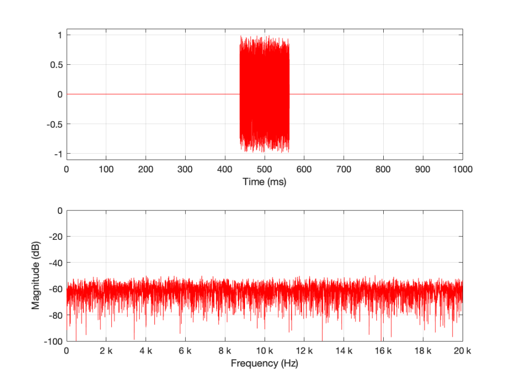
What happens if I have a one-second long signal, but only a portion of it is a burst of white noise, and the rest is silence? For example, look at Figure 5.
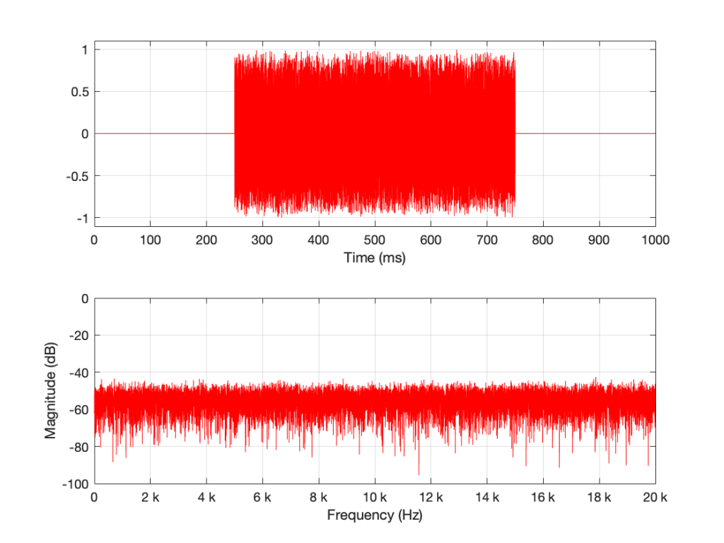
Figure 5’s magnitude response looks similar to the ones we’ve seen before (apart from being a little lower overall than the plots in Figures 1 and 3 – because there’s less energy overall in 0.5 sec of noise than there is in 1 second of noise). I’ll keep going to show what happens if we take this to an extreme.
The magnitude response shown in Figure 7 looks very different from the ones we’ve seen before. It’s much smoother… We’ll keep going…
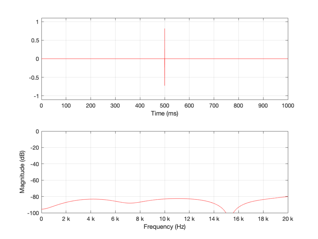
Figure 8 is very different again… The total magnitude response, even when not “zoomed in” is smooth. It’s important here to note that the actual response that we see there will be different every time I run the random generator again. For example, look at Figure 9, which is also a 16-sample long white noise signal.
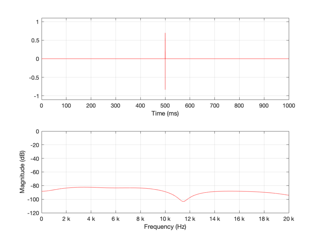
If we keep getting shorter and shorter, eventually we’ll get down to a single sample with a random value. However, since it’s a single sample (that is very probably non-zero) in a long string of zeros, then its magnitude response will be completely flat. It will not be noise – it will be an impulse with a random level. And it won’t sound like noise – it will sound like a click.
Summary
There are two basic important things to know at this point.
- White noise has the frequency content you expect only if you average over time.
- The shorter the time the noise is present, the less energy you will have, overall.
The discussion continues in Part 2.
P.S.
Thanks to David for emailing and pointing out that it’s “Hz” and “hertz” but not “Hertz”. I’ve corrected the text above… Being reminded of this reminds me of a Steven Wright joke – “I’m having amnesia and déjà vu at the same time. I think I’ve forgotten this before…”