I ended Part 3 by saying that DSP engineers think of the frequency scale as a circle rather than as a straight line. The questions are “Why do they think like this? What’s wrong with them?” Although I can’t answer the second question, the answer to the first question is fundamentally simple.
A DSP engineer is not really interested in what a filter does. She or he is interested in how it filters. A normal magnitude response plot shows us mortals the result of what’s happened to the audio after it’s gone through a filter (or a processor in general). Someone making that filter (or system) needs to know how it’s working instead.
So far, in this series, we’ve seen the following:
- Digital audio filters are made with feed-forward and feed-back delays with different gains.
- Feed-forward delays make narrow dips (and wide peaks) in the magnitude response
- Feed-back delays make narrow peaks (and wide dips) in the magnitude response
- DSP engineers think of frequency on a circle instead of a straight line
- DSP engineers also want to see plots of how a filter works instead of its result on the audio signal.
Let’s put all of this together.
We’ll draw the circle showing the frequency scale, but then rotate the view to see it in three dimensions. For example, I can pretend to make the surface of of the circle out of a rubber sheet that can be pulled upwards (like a tent) or downwards (like a funnel), whilst always maintaining a circular edge.
If I want to pull the tent upwards, I’ll use a “pole” to do it. That pole has an infinite height (we’re going to need some very stretchy rubber). If I want to pull the funnel downwards, I’ll use something I’ll call a “zero“. (I am not going to go into why zeros and poles are called that, so as to avoid doing too much math.)
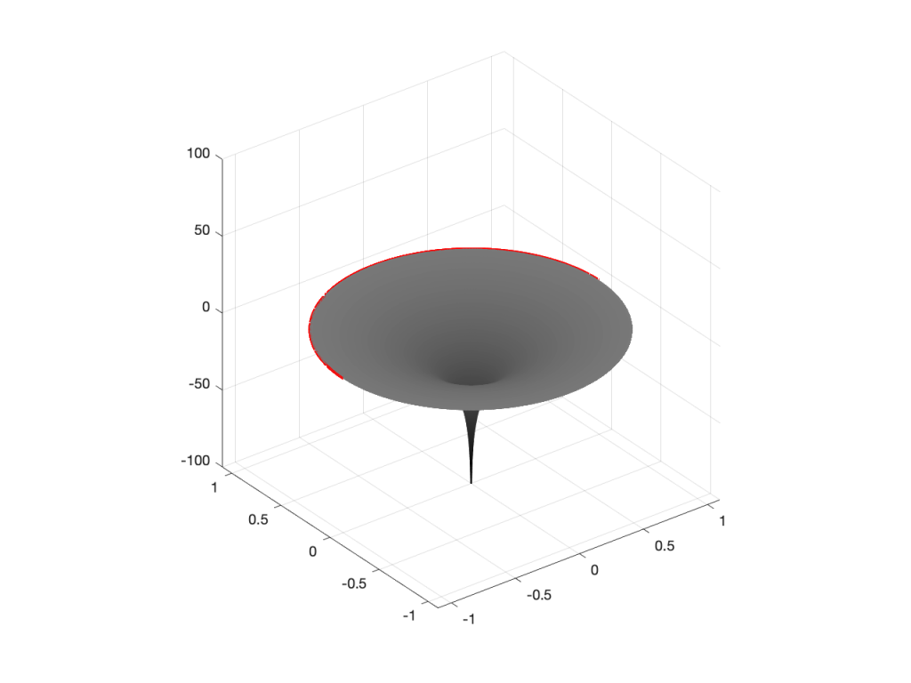
So, if I were to put a zero in the middle of the circle, its 2D representation would look like Figure 1 (notice the red circle in the middle showing where the zero is placed), and the 3D version would look like Figure 2:

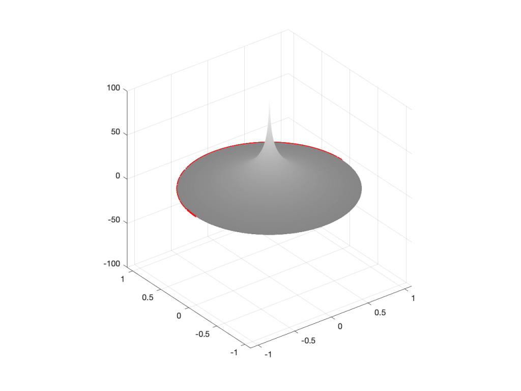
If I were to put the pole (indicated by a red ‘x’) in the middle of the circle instead, then the result would look like Figures 3 and 4.

So far so good… If we were to rotate Figures 2 or 4 and look at the red line that I’ve drawn around the edge, we’d see that it’s flat with a height of 0 (on the vertical scale) all the way around. This is because I’ve carefully placed the zero or the pole at the exact middle of the circle, so it’s pulling equally on all points of the edge of the “tent” or the “funnel”.
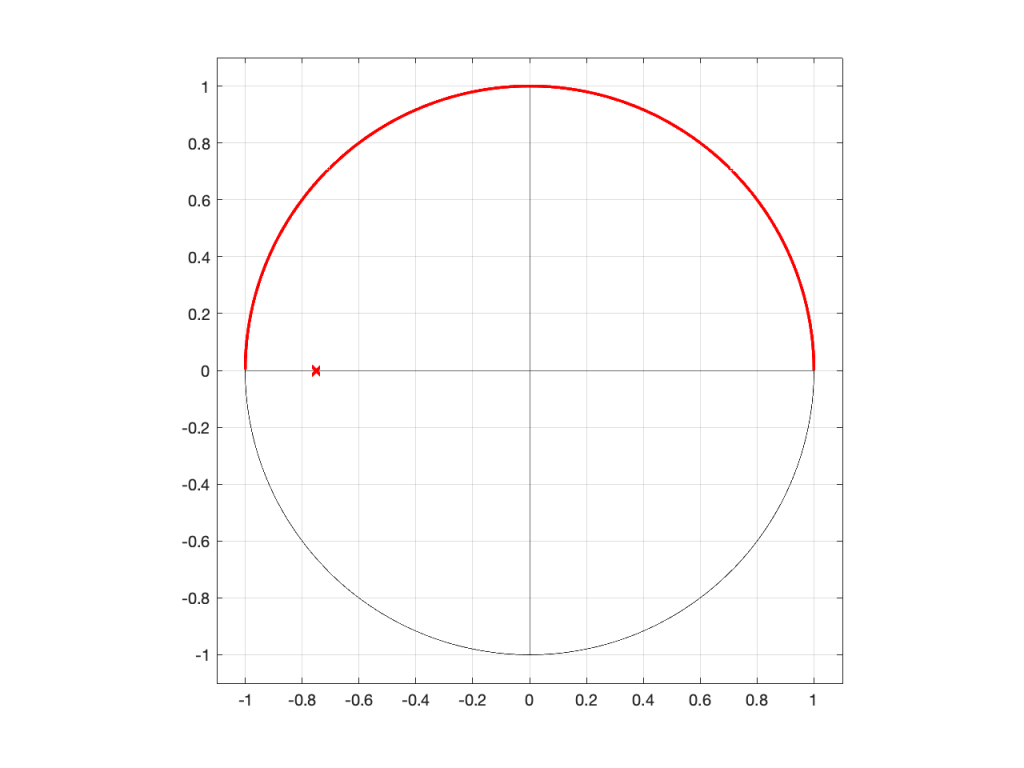
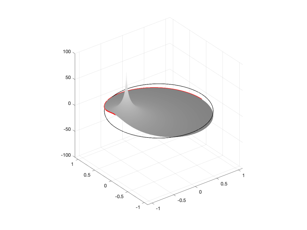
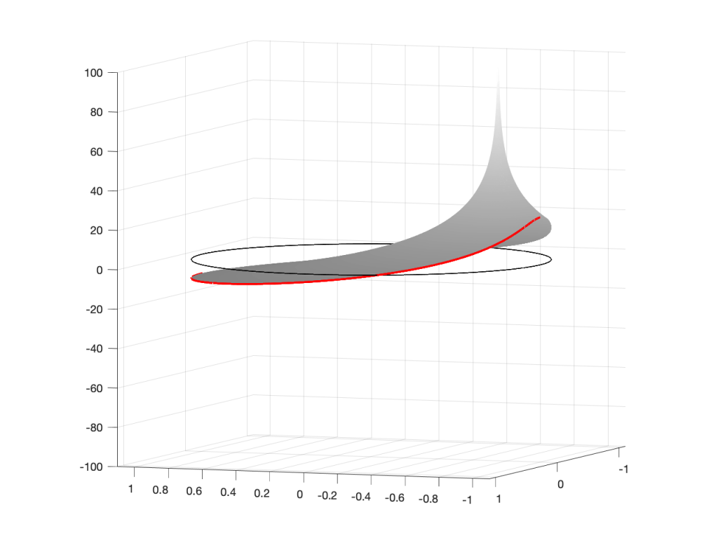
However, what would happen if I moved the zero or the pole away from the middle? Some examples of this for a zero moved to the location (-0.75, 0) are shown in Figures 5 to 7, below.
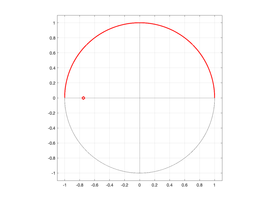
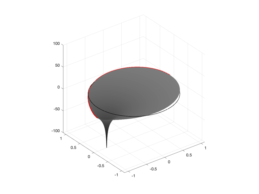
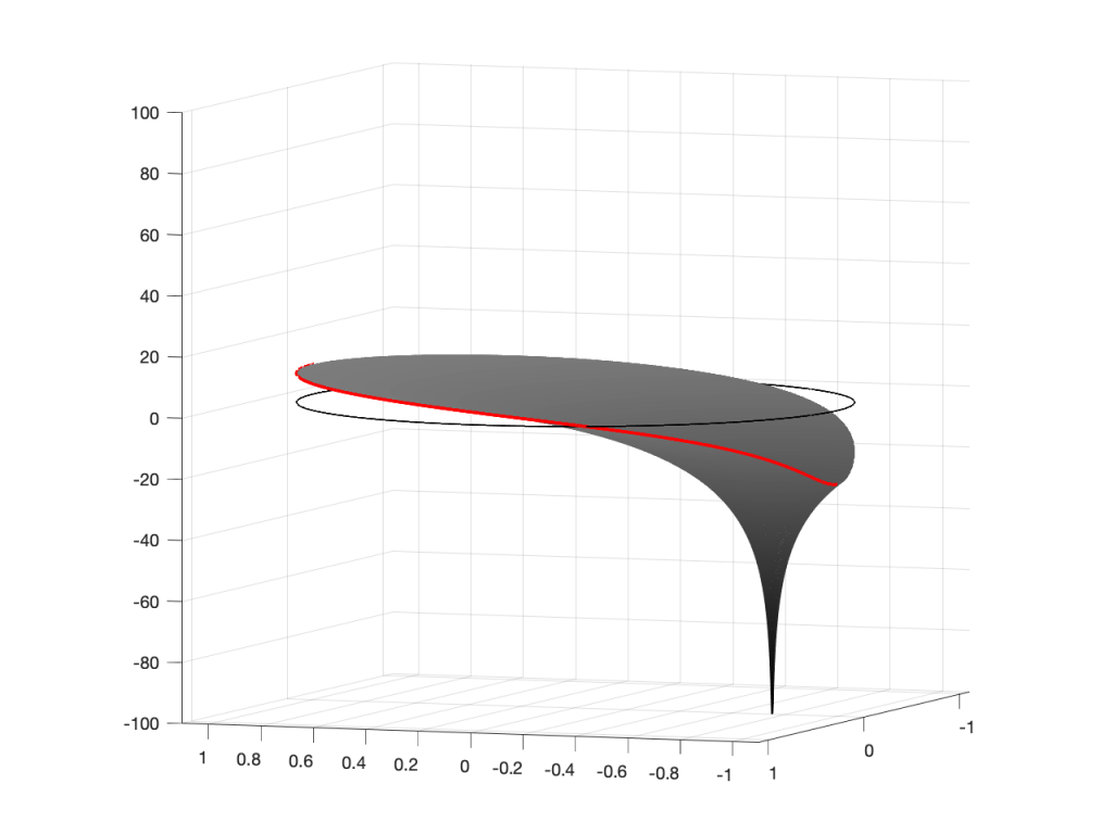
As you can see in Figure 7, when the zero is moved away from the centre of the circle, it pulls downwards on the closer edge (notice how the red line is lower than the black line which has a constant height of 0). However, it also doesn’t pull downwards as much on the opposite side of the circle (notice how the red line is higher than the black line on the left side).
Of course, if I were to do the same thing with a pole, everything would behave symmetrically, as shown in Figures 8 to 10.
We’re almost finished… One more posting to go to wrap up.