Previous parts in this series:
Resolution, Part 1: White Noise

When it comes to audio, the “signal” is an easy thing to define. It’s what you want to listen to – a song, the dialogue in the movie – whatever it was that you wanted to hear that made you turn on the loudspeaker in the first place.

Let’s say that, normally, we listen to music – so that’s the signal. And, although “music” means different things to different people, most of the time, “music” will contain energy at more than one frequency, and its level will change over time. For example, compare the two plots in Figure 1.

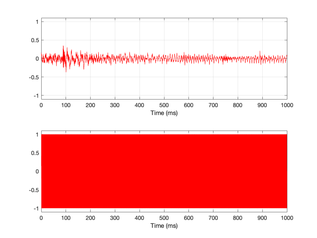
Looking at Figure 1, it seems obvious that the level of “Bird on a Wire” changes over time, but the level of a sine wave doesn’t. However, that’s not as obvious when we zoom into that plot, as is shown in Figure 2, below.

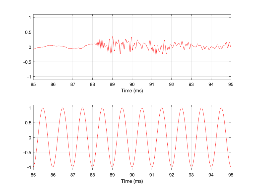
From Figure 2, we can easily establish the obvious fact that “Bird on a Wire” and a sine wave are different. However, now it’s not as obvious that the sine wave as a constant level – it repeats itself periodically – which is why we call it “periodic” – but what is its level?

The simplest way to determine the level of a signal is similar to the way yesterday’s share prices are shown in the financial section of the newspaper. In that case, you are told the highest price and the lowest price for the day. In audio, we sometimes talk to the “peak-to-peak” amplitude of a signal. This is the difference between the highest and and the lowest peak (more accurately called a “trough”) of the signal in whatever amount of time you’ve been measuring. For example, take a look at Figure 3.

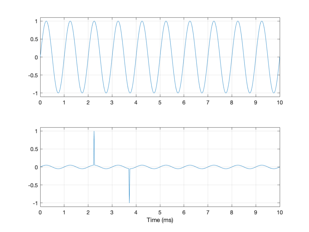
In Figure 3, I’ve drawn two signals. The top one is a 100 Hz sine wave with a peak-to-peak amplitude of 2 (because the difference between the highest peak (+1) and the lowest peak (-1) is 2). The bottom signal is a 100 Hz sine wave with a peak-to-peak amplitude of 0.1 – but with two clicks – one hitting +1 and the other hitting -1. So, if I just look at the peaks of that second signal, it also has a peak-to-peak amplitude of 2.

So, although it was easy to find the peak-to-peak amplitudes of those two signals, it should be obvious that this does not give a fair indication of how loud they appear to be.

However, if you’re building a piece of audio equipment (like an amplifier or an EQ, for example), this measurement does give you an idea of the “worst case” limits of the signal that might come through the system. So it’s not a useless measurement.

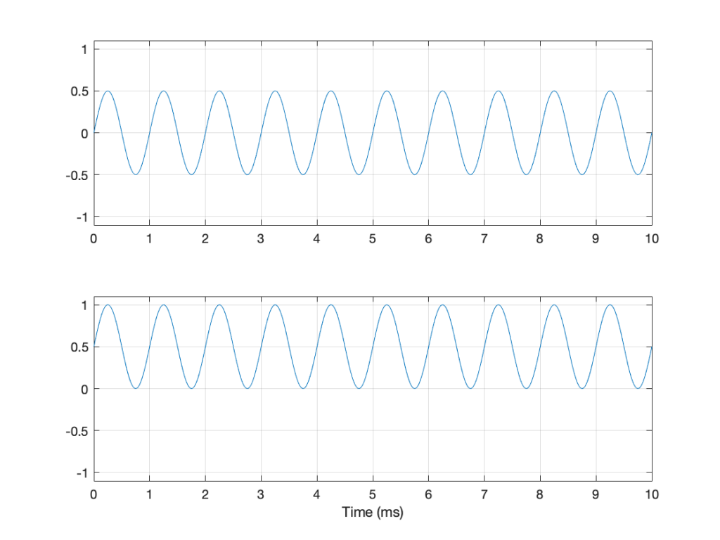
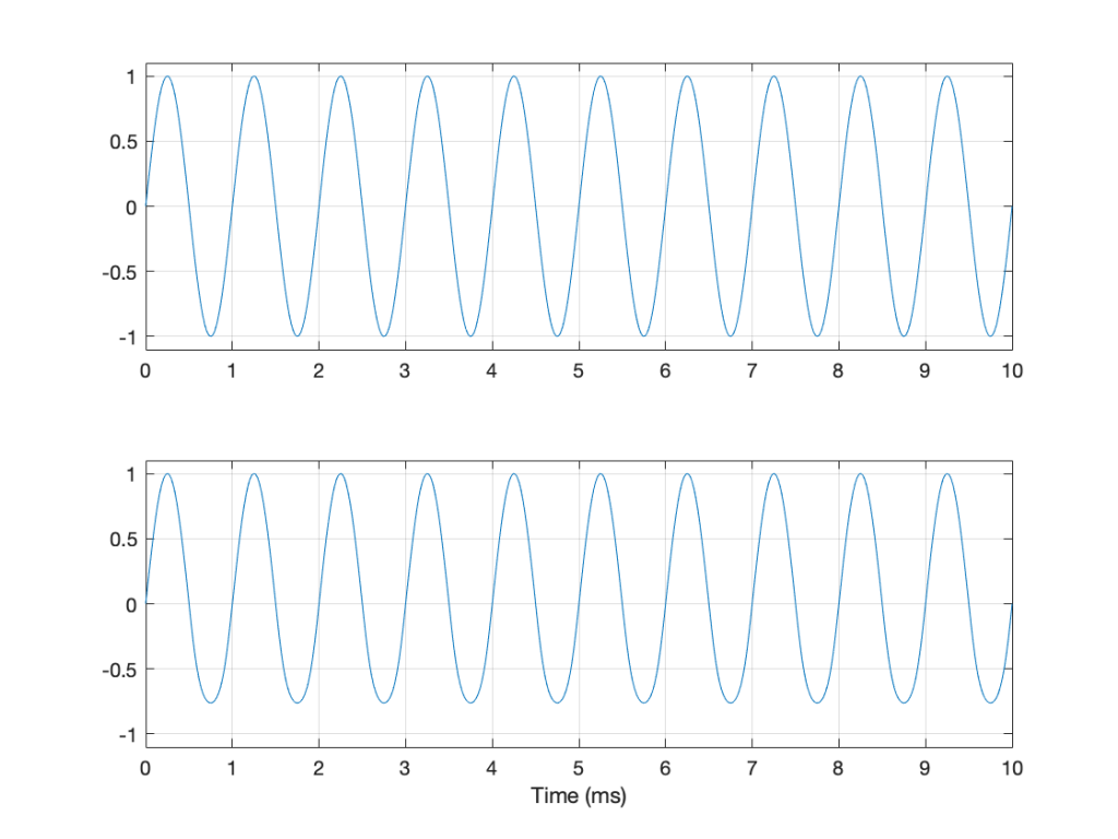
An additional problem with a peak-to-peak measurement of a signal is that it doesn’t tell you anything about asymmetry across the 0 line. (In an analogue world, we’d call that a “DC offset” because there would be a DC voltage that is added to the AC waveform.) For example, both of the signals in Figure 4 have a peak-to-peak amplitude of 1, but they are different…

If you’re lazy, you can do half of a peak-to-peak measurement. This is where you just check the maximum value of either the peak or the trough. We call this a “peak” amplitude measurement.

This has its problems, though. For example, take a look at Figure 5.

Here, we see two signals. The top one is a sine wave. The bottom one was a sine wave until I squished its negative-going half with a cheap compressor. As you can probably see, the top waveform is symmetrical – the negative half of the signal is the same as the positive half of the signal, just upside-down. It is also easily obvious that the second signal on the lower plot is not symmetrical. Its positive peak is higher than its negative peak.

However, both of these signals have a maximum positive peak of 1 – therefore their peak amplitudes are both 1 (but their peak-to-peak amplitudes and their apparent loudnesses are different).

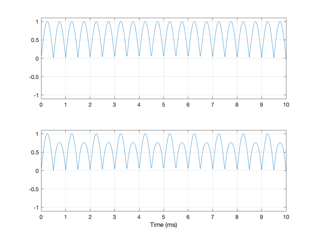
You might think that an easy way around this problem is to look at the absolute value of the signals and find the peaks that way. However, as you can see in Figure 6, in the case of asymmetrical signals, this does not change anything.

Another way to look at the signal is to take an average of the level over time. However, if the signal is symmetrical (like a sine wave, for example) this would not work, since the average will probably be 0. This is because, if the signal is symmetrical, then the average of all of the negative values in the signal (over time) average out to be the negative equal of the average of all of the positive values. So we can’t just use the average of the signal directly… However, with a little extra math, we can do something useful.

I’m going to skip quickly over some old-fashioned math here in order to jump to the punchline which is: “the power in an AC signal (like a sine wave) is proportional to the square of the signal.”

The reason for this can be explained by combining Ohm’s Law and Watt’s Law as follows:

V = IR

where V is electromotive force (or voltage) in volts, I is current in amperes, and R is the resistance in ohms.

P = VI

where P is the power in watts, and V and I are the same as above.

If we fiddle with Ohm’s Law like this:

V = IR

therefore

I = V/R

Then we can replace the “I” in Watt’s Law like this

P = VI

P = V * V/R

P = V² / R

So, with that last equation, we can see that the Power (in watts) is proportional to the square of the Voltage (in volts). So, if you double the voltage, you get 4 times the power (because 2² = 4).

We could do the same thing for current, as follows:

P = VI

P = IR * I

P = I² R

So what? Well, one thing this tells us is that, if you want double the power (for example, from a loudspeaker’s output or the heat from a hair dryer) then you’ll need 4 times the amplitude of the signal feeding it (for example, 4 times the voltage at the same current level or 4 times the current with the same voltage).

Now, let’s come back to the problem at hand… What’s the level of the signal? Well, we start by taking our signal and find its equivalent power (by squaring its instantaneous amplitude value over time – so, for example, if it’s a digital signal, we take the value of each sample and multiply it by itself). Part of the effect of this squaring of the signal is that it removes the negative portion of the signal (because a negative number multiplied by a negative number is a positive number).

We then take a slice of time, and average all of the values that we just created by squaring the original values. Now we have the average (or “mean”) power in the signal.

However, we’re not interested in the power of the signal, we’re interested in its “average” amplitude (say, its voltage). So, to get back from power, we take the square root of the average that we just calculated.

By doing all of this, we are finding the Root of the Mean of the Square of the voltage – the RMS level.

If we apply this math to a sine wave, the result will be something like what’s shown in Figure 6.

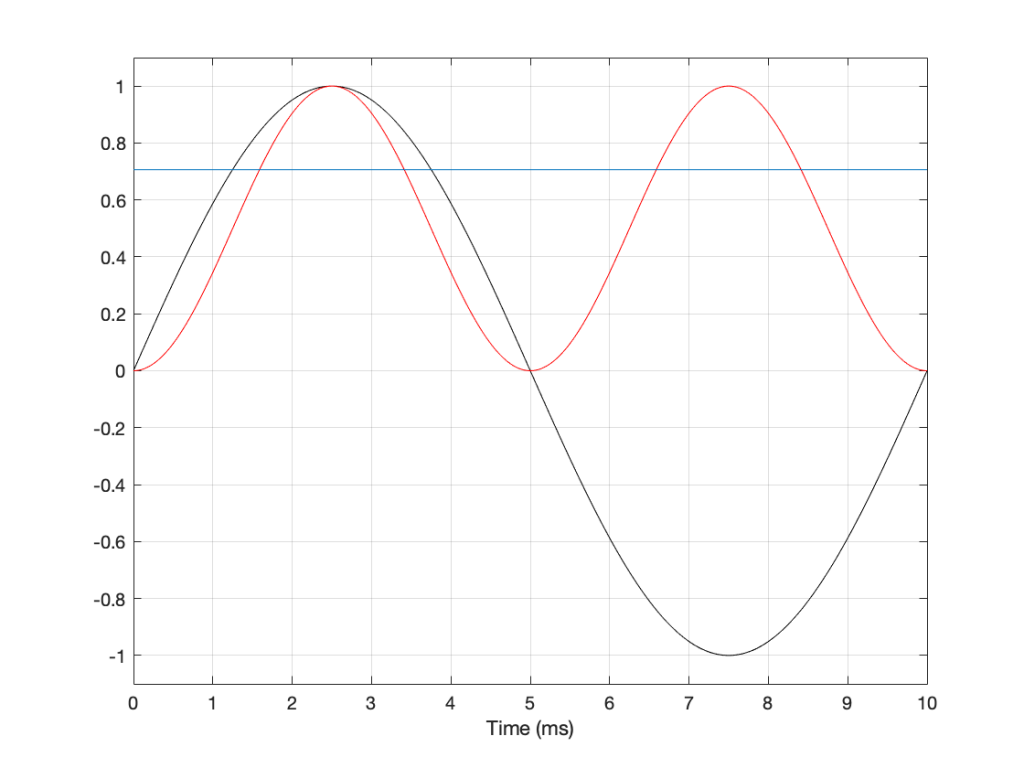
In Figure 6, the black curve is the original sine wave with a frequency of 100 Hz and a peak amplitude of 1.0 (and no DC offset). The red curve shows the result of squaring all the values in the sine wave (which is why it’s called a “sine squared” wave or sin² wave). If we find the average of all of the values in the red curve, the result would be 0.5. The square root of 0.5 is approximately 0.707 – which is shown as the blue line in the plot.

So, the RMS value of a sine wave with a peak value of 1 is 0.707. What does this mean? The easiest way to think of this is that if you had an old-fashioned incandescent light bulb and you powered it with a 1Vp (1 Volt Peak) AC voltage sine wave, it would be exactly the same brightness as if you connected it to a 0.707 V DC battery instead. If you wanted to use a battery to power your toaster, and you wanted it to make toast just as quickly as it normally does, then the battery will have to have a voltage that is 0.707 * the peak value of the AC voltage that normally feeds it. (Note that, if you live in North America, then the electrical signal feeding your toaster is 110 V RMS – so you’ll need a 110 V battery. If you live in Europe, then your toaster is fed with 220 V RMS – so you’ll need a 220 V battery. If you live somewhere else, you might need something else… Note that the electrical company has already done the RMS calculation for you…)

So, an RMS measurement of an AC signal tells us what DC value would result in the same power consumption.

There is just one problem: part of the RMS calculation is the “M” part – we are finding the mean of the values over some period of time. The length of time that we’re going to use is easy to choose if it’s a sine wave – we just make sure that the length of time (we call it a “time constant”) is at least as long as one period of the sine wave itself. If it’s smaller, then the RMS value will bob up and down as the sine wave goes up and down.

However, if we’re going to try to use the RMS method to find the level of a music signal, we’re going to have to make some tough choices… For example, let’s find the RMS value of the “Bird on a Wire” sample, using different time constants, shown below.

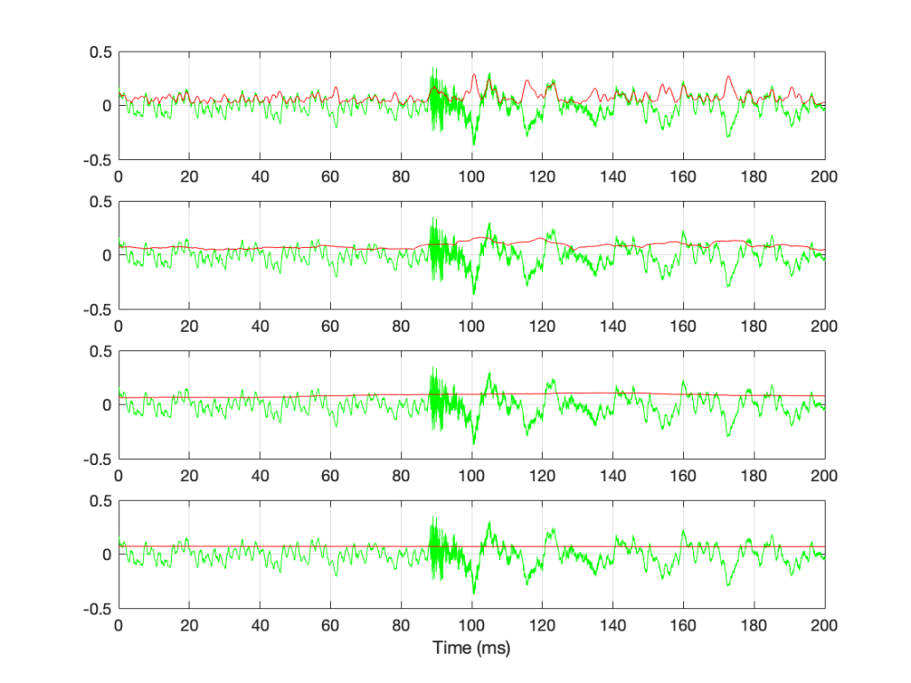
If we convert the plot in Figure 7 to a decibel representation by taking 20*log10 of each sample value, we get the plots in Figure 8. (Note that this is not the same as dB FS, since we are not comparing the result to the RMS value of a full-scale sine wave… but that’s a topic for another posting.)

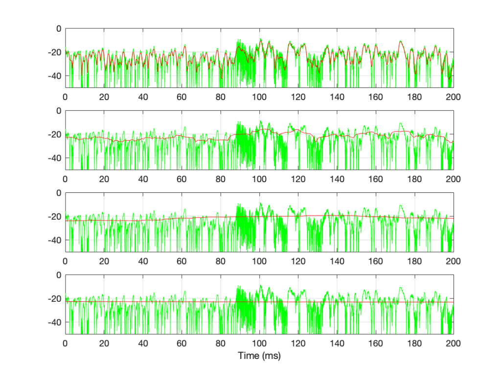
There are some things that are evident in Figure 8. The most obvious one is that there is a link between the RMS time constant and the variability of the RMS level when the signal that you’re analysing is not periodic. Looking at this short 200 ms-long example from Bird on a Wire, with the four time constants that I used, the range of results are as shown below in Figure 9.

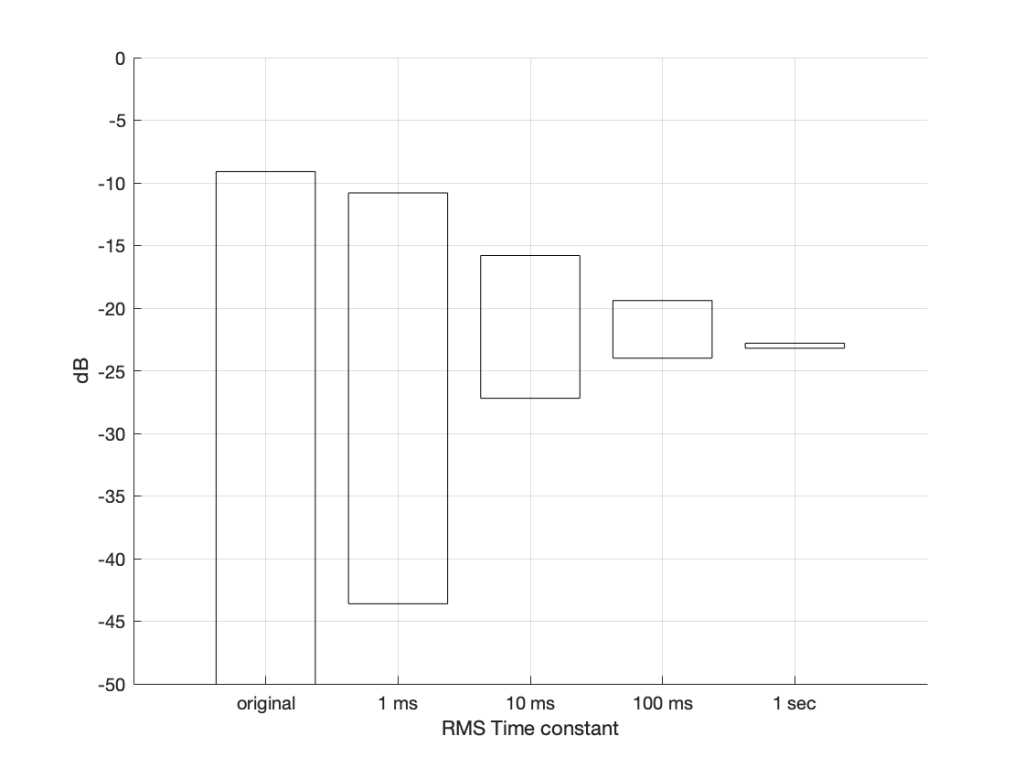
[table]

RMS Time constant, Min (dB), Max (dB), Range (dB)

Original signal, -∞, -9.1, ∞

1 ms, -43.6, -10.8, 32.8

10 ms, -27.2, -15.8, 11.4

100 ms, -24.0, -19.4, 4.6

1 sec, -23.2, -22.8, 0.4

[/table]

Of course, it’s important to remember that if I had picked a different signal or different RMS time constants, I would have gotten different results.

The question to ask here is:

“If I want to know the level of that 200 ms slice of Bird on a Wire, which RMS time constant should I use?”

or

“which of those four plots tells me the signal’s level?”

The answer is that none of these is correct – or all of them are, even though they show different things. The problem is that music has such a wide frequency range – from 20 Hz to 20,000 Hz. Therefore, if you choose a time constant that is long enough to give you a stable measurement at 20 Hz (which will be at least 50 ms – 1/20th of a second or one period of a 20 Hz wave), then it will be the length of 1000 periods of the 20 kHz portion of the signal.

Of course, you could argue that you care more about the 20 Hz part than the 20,000 Hz part – but that’s dependent on what you’re doing. If you’re measuring the signal that’s being sent to a tweeter, then you’re probably not interested in what’s going on at 20 Hz at all…

So what?

We’re heading (in a future posting) towards talking about measuring a system’s (or a devices’s) ability to deliver a wide range of signal levels. We’re going to talk about its “signal to noise ratio” which is a measurement of how much louder the signal (the music) is than the noise that the system itself generates. The idea in the design of all audio systems is that you want to make that ratio as big as possible so that you cannot hear the noise because it’s so much quieter than the signal.

The problem is that we’re going to have to measure how loud the signal can be – and compare that to how loud the signal actually is at any given moment. In order to understand the concepts in that discussion, then it’s necessary to understand the concepts that I introduced above, namely the following:

• Peak-peak level
• Peak level
• RMS level
• the relationship between RMS Time constant and the RMS level