In a previous posting, I tried to explain the concept of aliasing. The easiest way to illustrate this is to try to sample an audio signal that has a frequency that is higher than the Nyquist frequency – one half of the sampling rate. If you do this, then the signal that will come out of your digital audio system will have a different frequency than the original signal. In fact, it will be the Nyquist frequency minus the difference between the original signal and the Nyquist frequency.

For example, if we have an LPCM audio system that has a sampling rate of 48 kHz, then its Nyquist frequency is 24 kHz. If you allow any audio signal to be sampled by that system, and you record a sine wave with a frequency of 30 kHz, then the signal that will be played back by the system will be

Nyquist – (signal freq – Nyquist)
24 kHz – (30 kHz – 24 kHz)
24 kHz – 6 kHz
18 kHz

Digging a little deeper

The example I gave above is only part of the story. It’s the part of the story that’s told because it’s easy to tell, and relatively easy to grasp. However, let’s look into this a little more…

If I ask you “what is the square root of 4?” you’ll probably say that the answer is “2”. However, this is also only part of the story. The square root of 4 is also -2, since -2 * -2 = 4. So, there are two correct answers to the question – in other words, both answers exist and are equally valid.

Aliasing is somewhat similar. If we manage to get a 30 kHz sine wave into an LPCM recording system with a sampling rate of 48 kHz, we will appear to have recorded an 18 kHz sine wave. However, the samples that we have captured are also equally valid for the original 30 kHz sine wave. In fact, both the 18 kHz and the 30 kHz tones can be thought of as being equally valid answers to the set of samples we recorded.

This means that, if I record an 18 kHz sine tone in the 48 kHz system, we can consider the 30 kHz sine tone to also exist simultaneously, inside the digital domain.

Oddly, this is also true at other frequencies. So, you do not only get a mirror effect around the Nyquist, but you also get it at the 1.5 times the sampling rate (or the sampling rate + Nyquist).

I won’t go into this any deeper for now – but if you want to continue, the section on “Folding” at the Wikipedia page on Aliasing is a good place to start.

 

Normally, we try to prevent audio signals higher with frequency content higher than the Nyquist frequency from getting into an LPCM system. This is done by low-pass filtering the audio signal to eliminate any content that might cause aliasing. That’s why the low-pass filter at the input of an analogue-to-digital converter is called an anti-aliasing filter. (At least, that’s the theory. In reality, the anti-aliasing filter of many ADC’s allow a little signal to get through above Nyquist…)

However, what happens if you create signals with a frequency above the Nyquist within the digital domain? Is this possible? Can it happen accidentally?

The short answer to this question is “yes”.

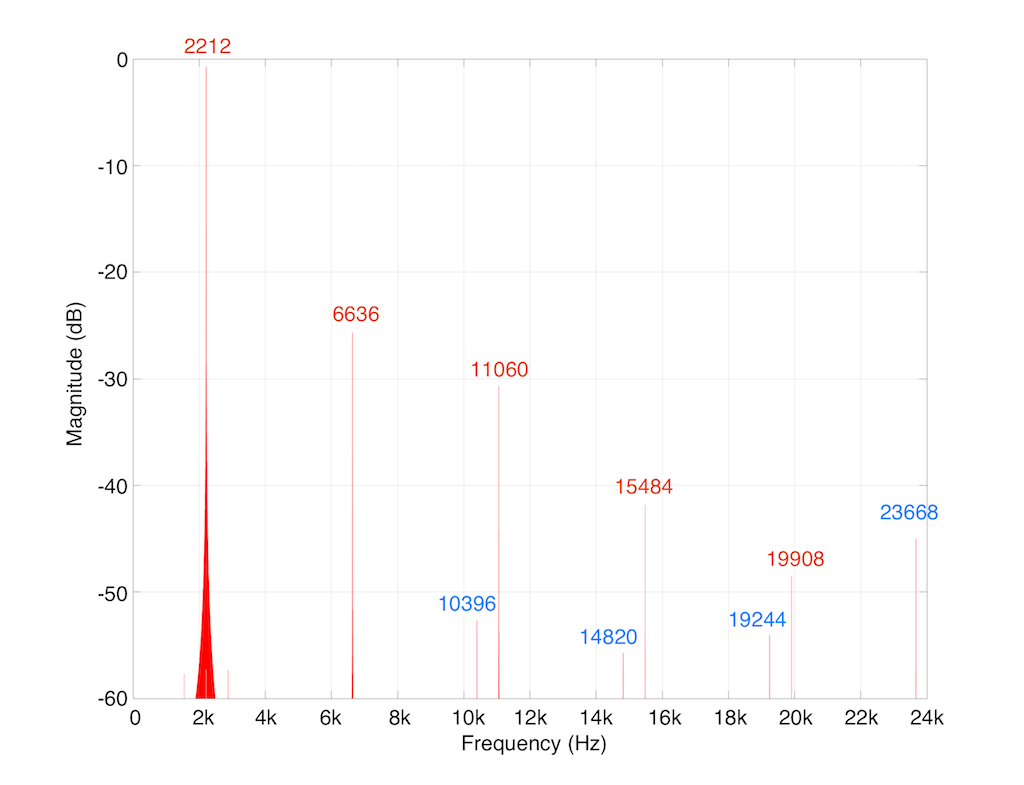
For example, let’s take a sine wave with a frequency of 2212 Hz (this is an arbitrary number… it could have been something else…), record it with an LPCM system with a sampling rate of 48 kHz. Then, after the signal is in the digital domain, I clip it at 85% of the peak value, so it looks like the waveform shown in Figure 1.

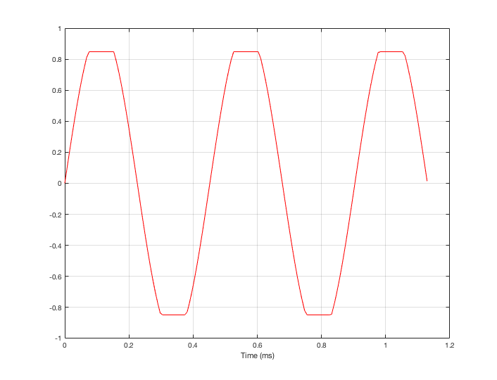
By clipping the sine wave symmetrically (meaning that we have made the same change in the wave’s shape on the top and the bottom), we create odd-order harmonics. This means that, when we look at the spectrum of the signal’s frequency content, we will see energy at the fundamental frequency (the original sine wave’s frequency) and also peaks at 3x, 5x, 7x, 9x, that frequency – and so on.

(If I had clipped only on the top or the bottom, and therefore made asymmetrical distortion, we would see energy in the even-order harmonics at 2x, 4x,  6x, 8x, the fundamental frequency – and so on.)

So, let’s look at the frequency content of the clipped signal shown in Figure 1. This is shown in Figure 2, below.

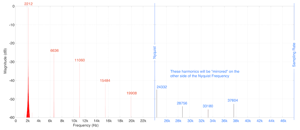
As you can see in Figure 2, we are expecting to see harmonics that extend (at least in this plot) up to 37604 Hz (or 17 x 2212 Hz). Of course, there are harmonics that go higher than this – but they aren’t visible in this plot because I’m only plotting signals with a level down to -60 dB FS.

You may notice that the width of the plot at 2212 Hz increases at the bottom. This is just an artefact of the math being done to find the frequency components in the signal. That spread in the frequency domain isn’t actually in the signal itself, so it can be ignored.

As I said above, the signal was clipped in the digital domain, in an LPCM system running at 48 kHz. So, just for reference, I’ve put in blue lines in Figure 2 that show the sampling rate and the Nyquist frequency – one half the sampling rate.

So: we can see that some of the artefacts created by clipping the signal are sitting at frequencies above the Nyquist frequency in this system. This means that this content will be “mirrored” or “folded down” or – more correctly – aliased to other frequencies below the Nyquist frequency. For example, the harmonic at 24332 Hz will be mirrored to 23668 Hz, according to the following math:

Nyquist – (signal freq – Nyquist)
24000 – (24332 – 24000)
24000 – 332
23668 Hz

So, looking at the top 60 dB of the signal content (shown in Figure 3): the resulting actual output of the LPCM signal will contain:

1. the original fundamental frequency at 2212 Hz
2. four harmonics of that frequency (shown as the other red numbers in Figure 3), and
3. four more frequencies that are not harmonically related to the fundamental (the blue numbers)

 

As you may already know, an LPCM system has a low-pass filter at its output stage – part of the system that is used to convert the signal back to an analogue output. However, that low pass filter typically has a cutoff frequency around the Nyquist frequency of the system. However, the artefacts that we have created here have aliased down to frequencies below the Nyquist within the digital domain – so, by the time the signal reaches the low pass filter at the output (known as a “reconstruction filter”) they’re already in the audio band, and therefore they’re not filtered out.

So, as we can see in this rather simple example: it is easily possible that a digital audio system that has some processing (specifically “non-linear” processing) can create harmonics that are higher than the Nyquist frequency and will have “aliases” below the Nyquist frequency, and therefore will not be removed by an anti-aliasing filter.

Since the aliased artefacts are not harmonically related to the fundamental frequency, they are more easily audible than “normal” distortion artefacts that generate harmonically-related artefacts. There are a couple of reasons for this, but the most obvious one can be demonstrated by sweeping the frequency of the fundamental. If the artefacts are harmonically related, then as the fundamental frequency of the signal goes up, so do the artefacts. However, if the artefacts are the result of aliasing, then as the fundamental frequency of the signal goes up, some of the artefacts go down in frequency, which sounds quite strange…

The example I gave above (of clipping) is just one way to create distortion that generates harmonically-related artefacts that alias in the system. Lots of different processes can create those artefacts. One of the usual suspects is a poorly-made sampling rate converter.

Many systems use sampling rate converters for different reasons. For example, if you have a loudspeaker or processor that has a lot of filtering in its processing chain, the best architecture is to run the digital signal processing (the  DSP) at a constant (or “fixed”) sampling rate, regardless of the sampling rate of the incoming signal. This is because, if you were to change sampling rates in the DSP to match the incoming signal, you would have to load an entirely new set of coefficients (a fancy word that basically means “multiplications values inside the digital filters”) into the processor. This takes some time, and you don’t want to miss the first part of the song every time the sampling rate changes while you’re waiting to load a bunch of new coefficients into your filters… So, instead, the smart thing to do is to keep the DSP running at a constant rate, and sample rate convert all incoming signals to the internal sampling rate. This way, there’s no dropout at the start of the song.

However, you have to be careful if you do this, since a poorly-made sampling rate converter will certainly create aliasing artefacts.

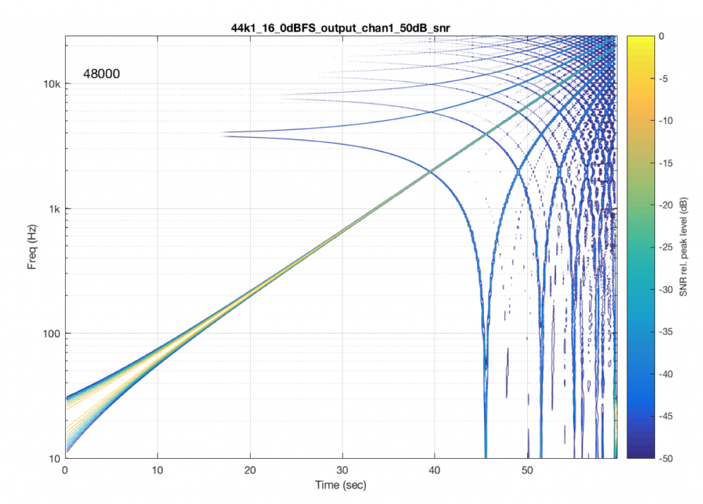
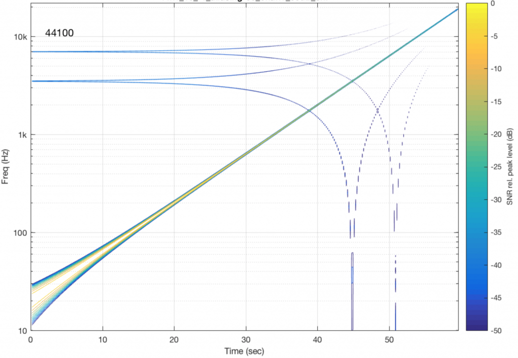
In part 5 of this series of postings, I described one kind of test that can be made on an audio system. This test consists of sending a sine wave with a swept frequency into the system and recording its output. You then do a spectrogram of the output, looking for signals at frequencies other than the one you sent in.

To get an idea of what aliasing will look like in this plot, I made a DSP algorithm that creates the same kinds of artefacts. The resulting plot is shown in Figure 4, below. (Remember that this is a measurement of a system that I made to intentionally generate similar artefacts to aliasing – this isn’t actually the output of a system that is aliasing).

 

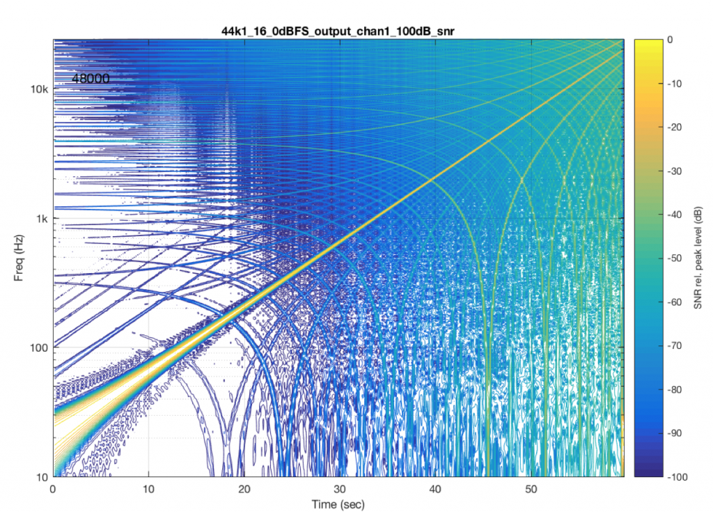
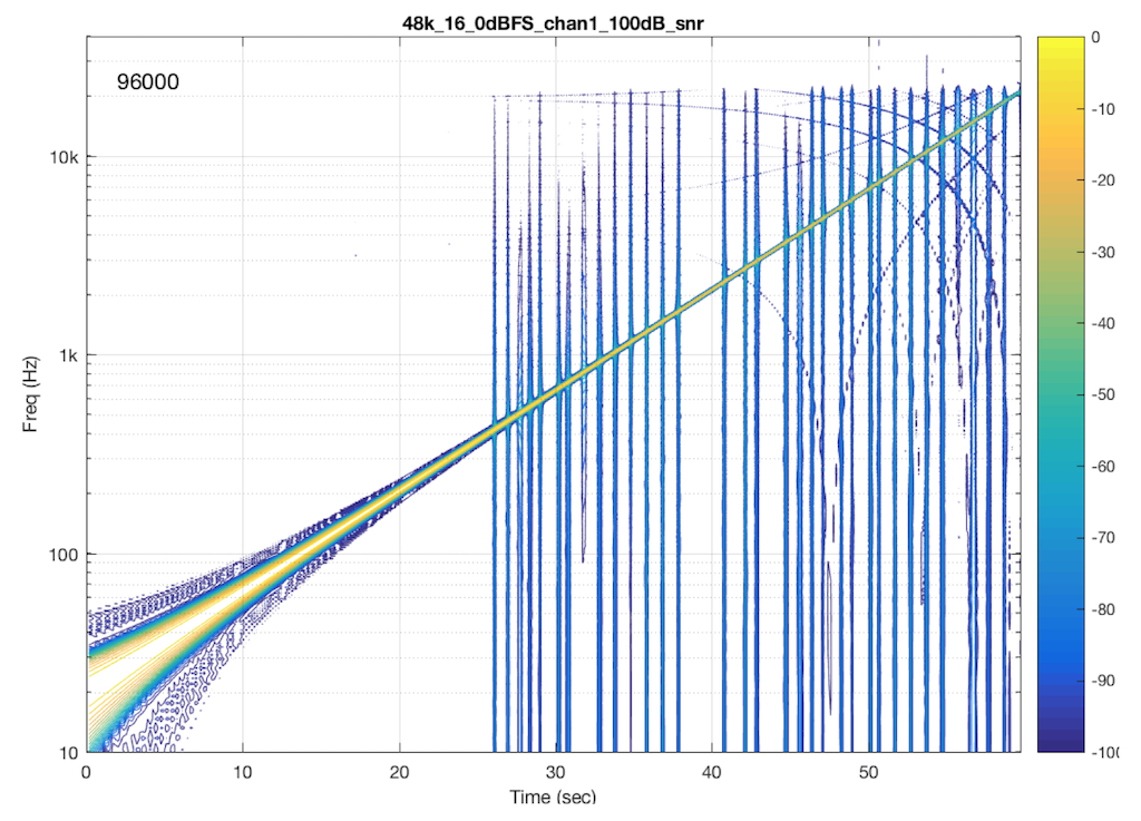
Now that you know what to look for in the plot, let’s look at the measurements of some commercially-available systems. Figure 5, below is a measurement of a system that has two problems. One can be seen as the vertical lines – these are “skip/insert” artefacts that I described in an earlier posting. The aliasing artefacts can also be seen in this plot. Note that, in this case, the input and output of the system are both digital connections to my measurement equipment.

 

 

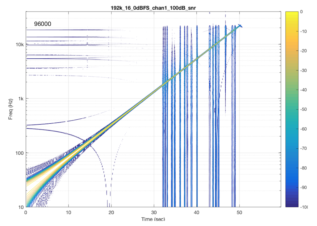
If I send a signal at a different sampling rate into the same system, I get a different behaviour. This is not unusual in systems with sampling rate converters. In this plot, you can see the skip/insert artefacts (the vertical stripes) the aliasing artefacts, and the obvious band-limiting of the system. Notice that nothing above about 24 kHz comes out of the system, which would mean that, internally, it is probably running at a sampling rate of 48 kHz. (The input signal in this measurement was at 192 kHz and my analysis system was running at 96 kHz.)

Let’s look at another system. In this case, I put a 48 kHz, 16-bit .flac file on a hard drive, and played it through another digital audio system, again capturing its digital output. The result of this is shown in Figure 7.

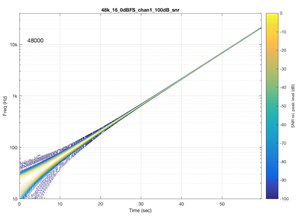
As you can see in Figure 6, this system is behaving very well in this particular test. I see the nice, clean signal with only one frequency at only one time. No artefacts down to 100 dB below the signal level. This is good.

Now let’s test exactly the same system, at exactly the same sampling rate, again with a .flac file – but this time with a 24-bit word length in the file. The result of this is shown in Figure 7.

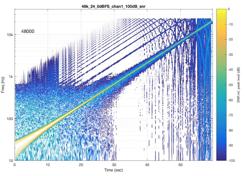
So, by going from a 16-bit file to a 24-bit file, this system obviously behaves very, very differently. It now has harmonic distortion (the straight diagonal lines running parallel to the fundamental frequency), aliasing of those harmonics when they go beyond 24 kHz, and strange noises as well (the large area of blue blobs in the lower left corner, and surrounding the fundamental frequency all the way up.

Those “strange noises” –  the blobs – are probably artefacts caused by a lossy codec similar to MP3. Typically, systems like this are built to reduce the data rate of the audio signal by trying to predict what you can’t hear in the signal – and leaving that out. In doing so, they create errors that produce noise, so the encoder tries to shape that noise so that it “hides” under the signal that it keeps. The end result looks something like the blobs shown in Figure 7… For a more thorough discussion of this, see this posting.

So, based only on the information from this test, we can guess that the system might be decoding the 24-bit file, “transcoding” it to a lossy format, and transmitting that through the system. However, this is just a guess based on one test… So it could easily be wrong.

One thing we can conclude, however, is that the 48 kHz / 16-bit file behaves MUCH better than a 48 kHz / 24-bit file in this system… So, in this particular case, a higher resolution is not necessarily better…

I should also point out that the digital output of that system was capable of outputting 24 bits. The reason I’m pointing this out is that many persons think that if a system or device has a digital output, then it is good. This is too simple a conclusion to make, because, as I’m trying to illustrate with this series of postings, the “weak link” in the chain is very likely NOT the physical output of the system. It’s more likely some part of the processing in the DSP chain (for example, a poorly-made sampling rate converter that aliases) or a poorly-implemented clocking system (for example, a skip/insert strategy).

For more aliasing fun…

If you’re intrigued by this, and you’d like to compare the aliasing caused by other sampling rate converters, I’d recommend checking out the page at http://src.infinitewave.ca. They plot the signals with a linear frequency scale instead of a logarithmic one. Consequently, the sweep of the fundamental looks like a curve (instead of the straight lines in my plots) but the harmonic distortion and aliasing artefacts are easier to see as being related to the fundamental.

 

Addendum – 2018/05/14

Last week, I ran a quick test on another commercially-available device – this time, a stand-alone audio file player with a digital output. I was running the test using a 44.1 kHz, 16-bit FLAC file, but the device had a 48 kHz output. The interesting thing about this one was that the artefacts that showed up were almost exclusively aliasing errors. So, I thought it would be interesting to show the plots here.