In this posting, we’ll do something similar to the analyses from Part 7. In that one, we
took two point-source theoretically perfect loudspeaker drivers (which means that they have the same magnitude response in all directions in 3D space), (pretending that they were a tweeter and a woofer in a non-existent cabinet)
filtered each of their inputs using a crossover network
separated them by some distance
measured them in a bunch of places on a sphere surrounding the non-existent cabinet
found the total magnitude response of the system when measured all around on that sphere, which is called the loudspeaker’s Power Response.
Now, we do that again, but we will include the real loudspeaker drivers’ measurements in that three-dimensional world. In this case, we still have the 1″ tweeter and the 6″ woofer in a sealed cabinet. Those two loudspeaker drivers were individually measured at 130 points around them on that sphere that I showed in Part 7.
I then take each of those 130 measurements for each driver, filter them using the crossover, and add the two outputs together, which gives me a total response for each location. I can then find the total response which gives me the Power Response of the two-way loudspeaker with two real loudspeaker drivers in a real cabinet, with the 5 different crossover types that we’ve been talking about.
Note that I have NOT done what I said I SHOULD do at the end of part 9. I have just been dumb and stuck the crossovers in front of the loudspeaker drivers without thinking about modifying the filters to compensate for the drivers’ characteristics.
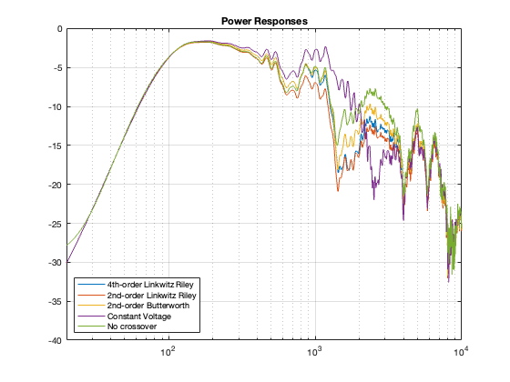
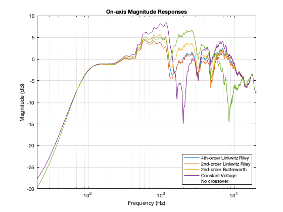
The five resulting power responses are shown in Figure 10.1.
Figure 10.1
The first thing to notice is that there is a roll-off in the low end. This is the natural response of the woofer that we saw in Part 9.
The second thing that you’ll notice is the general downward-slope of the plot, starting at about 100 Hz and having a generally decreasing magnitude the higher you go in frequency. This is the result of “beaming”. Since the two loudspeaker drivers, generally, have less and less high-frequency output as you move off-axis, then this appears as less total output from the system on that sphere. If the two loudspeakers were omnidirectional, then the power response would be a horizontal line. The more directional the drivers, the steeper the downward slope of this plot.
Now remember back to Part 7, where we did a little trick where we made an assumption that a person building or installing a loudspeaker would measured its on-axis response, and then put in an equaliser to flatten this measured response.
In the old days, you would do this “by eye” using something like a graphic or a parametric equaliser. But nowadays, we have fancy tools that can do measurements and create complicated FIR filters that do whatever we want. This means that we can REALLY screw things up with the precision of a surgical scalpel…
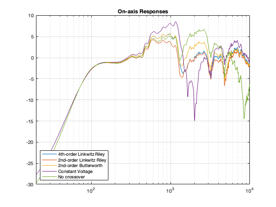
So, let’s be dumb and do the same thing again. We’ll take the on-axis responses of the loudspeaker with the different crossovers (we already saw these in Part 9, but here they are again, shown in Figure 10.2), and we’ll make five “perfect” equalisers that make each of these five responses perfectly flat.
Figure 10.2
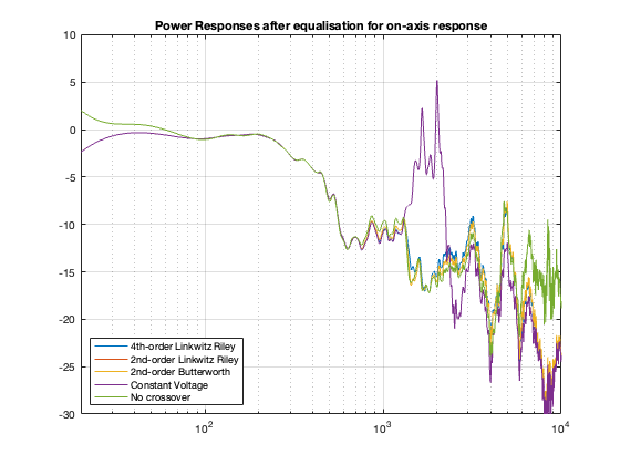
After applying each of these customised filters that make our on-axis measurement look like a laser beam, we should probably check what happened to the power responses. They’re shown below in Figure 10.3.
Figure 10.3
As you can see there, the low frequency response flattens out. This is because we’re really boosting the bass (to fix the on-axis measurement) and this loudspeaker happens to be fairly omnidirectional below about 200 Hz.
You can also see that I was REALLY dumb when I made those equalisation filters. For example, the notch in the on-axis response of the Constant Voltage caused me to make a horrendous peak that results in a really nice-looking plot at one on-axis point in space, but completely messes up the response of the loudspeaker in almost all other directions, resulting in that giant 15 dB peak around 2 kHz (remember that our crossover frequency is in this region…). The moral of this story is “don’t fix the on-axis response without considering the power response”. OR “just because it looks flat doesn’t mean that it’ll sound good.” On the other hand, notice that, after equalisation, most of the other curves look pretty similar-ish which means that maybe doing some intelligent equalisation for the on-axis response isn’t necessarily a bad idea.
Remember, however, that we’re still only looking at the loudspeaker in infinite space. There’s no room “singing along” with this loudspeaker… but the topic of room compensation is for another time…
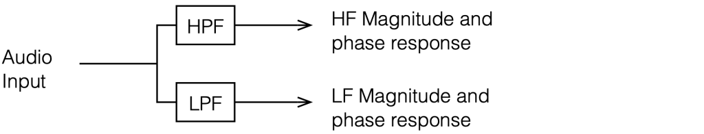
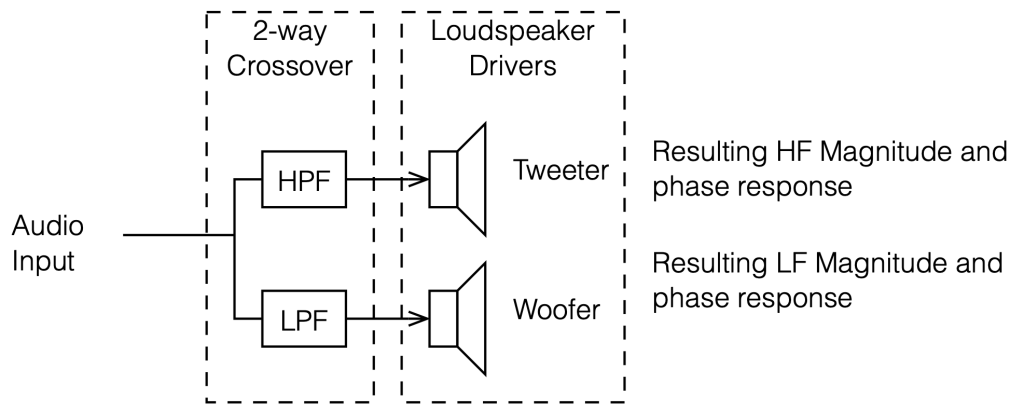
Up to now, we’ve either assumed that we don’t have any loudspeaker drivers in the chain (Parts 1 to 5 inclusive) or that our loudspeaker drivers are “perfect” point sources (Parts 6 to 8 inclusive). This means that, so far, our nice, perfect world has used a model that looks a little like Figure 9.1
Figure 9.1.
Now, we start getting a little closer to reality by adding some actual loudspeaker drivers to the outputs of the crossover. Going forward, I’m using the actual measurements of a real 1″ tweeter and a real 6″ woofer in a real sealed cabinet. So, now, instead of just looking at the magnitude and phase responses of the crossover’s outputs, we’re looking at the responses of the outputs of the drivers, as shown in Figure 9.2. Another way to think of this is that we have extra filters (the drivers’ responses, which are different in different directions) in addition to the filters in the crossover.
Figure 9.2
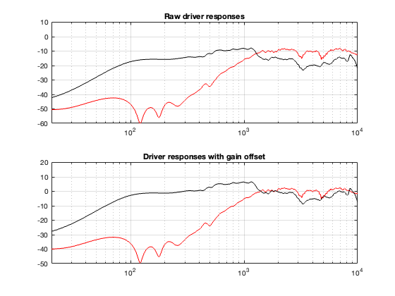
The problem with real loudspeakers is that they aren’t perfect, so let’s start by looking at their responses on-axis. These are shown in Figure 9.3
Figure 9.3.
The top plot of Figure 9.3 shows the on-axis magnitude responses of the loudspeaker drivers in the cabinet without any filtering. The bottom plot shows the same responses, with gain offsets to match them at an arbitrary crossover frequency of 1800 Hz.
4th Order Linkwitz Reily
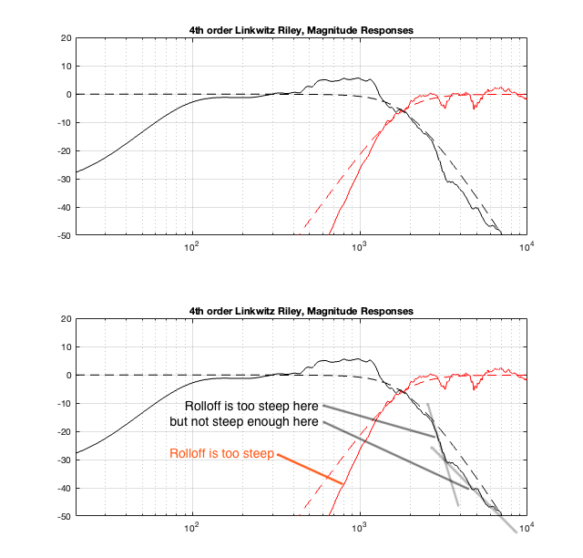
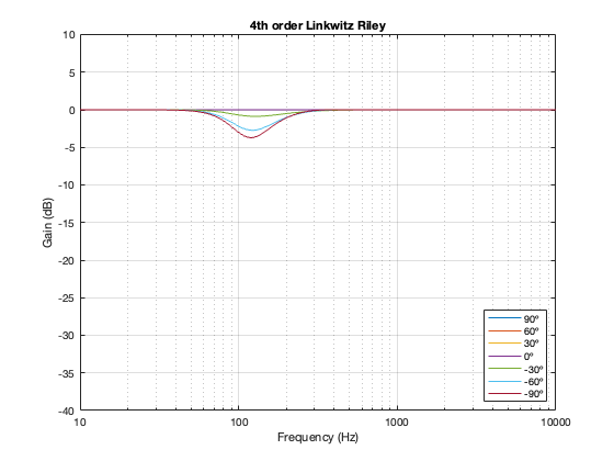
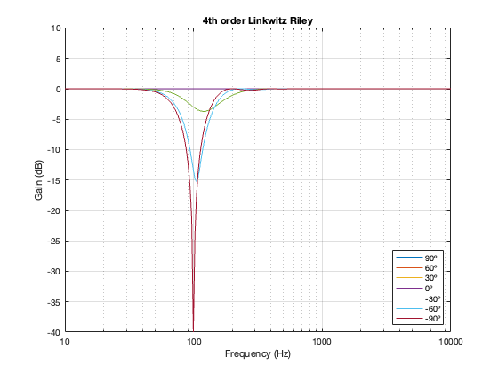
If I apply filtering using a 4th-order Linkwitz Reily crossover, and then send its outputs to a tweeter and a woofer, the resulting magnitude responses of the two drivers, when measured on-axis to the cabinet will look like the top plots in Figure 9.4, below.
I’ve duplicated the plot in the bottom half of the figure, and added some comments. Notice that the responses of the actual loudspeaker outputs, including the crossover filter, do NOT look like the theoretical responses of the crossover itself (shown as dotted lines). On-axis, the tweeter has a natural high-pass characteristic (seen in Figure 9.3) that, when combined with the high pass filter in the crossover, results in a slope that’s too steep.
The woofer’s rolloff is weird in that its contribution makes the low pass filter too steep at the start of the rolloff, and then not steep enough as you get a little higher in frequency. If you look back to Figure 9.3, this can be seen as the dip in the response that produces the “bowl” shape from roughly 1 kHz to 8 kHz.
Figure 9.4.
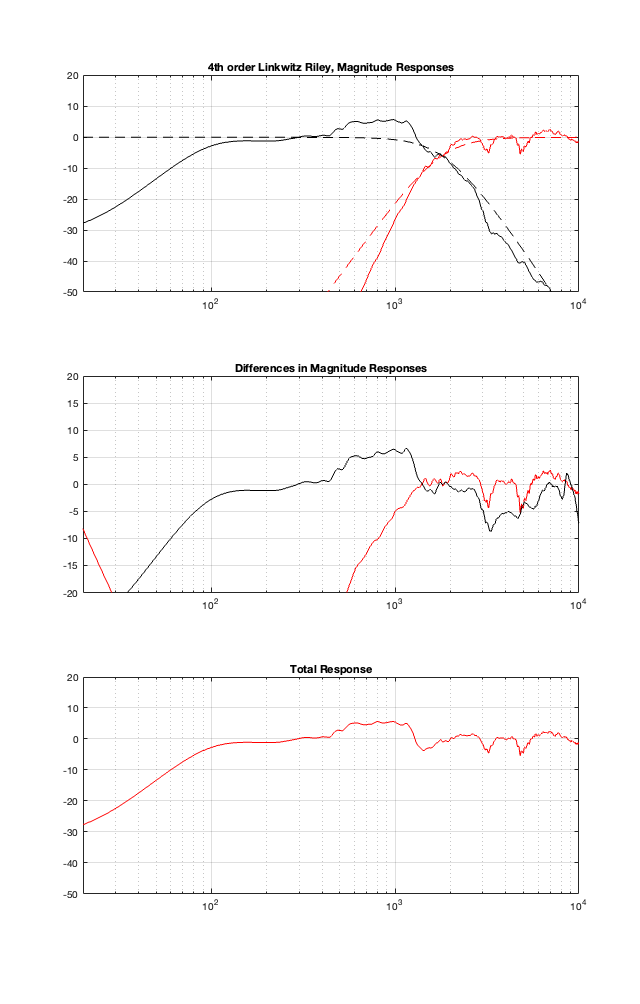
This means that, if we ignore the natural on-axis magnitude and phase responses of the loudspeaker drivers, and just slap a crossover in front of them, the resulting total response won’t be as pretty as we would expect. This is shown in the bottom plot in Figure 9.5.
The plots shown in the middle of Figure 9.5 are the difference between what we WANT the crossover to be (the dotted lines in the top plot) and the ACTUAL total resulting magnitude response at the outputs of the drivers (the solid lined in the top plot). In other words, these curves show the vertical distance between the solid and dotted lines in the top plot. If the drivers had perfectly flat magnitude responses, then these two lines would be flat, and they would sit on the 0 dB line.
Figure 9.5.
You might say that the Total Response in Figure 9.5 looks pretty good. I would disagree. An on-axis in-band magnitude response of about ±5 dB is pretty terrible if your goal is a flat on-axis response. If this is not your goal, then I have no opinion.
Now I’ll just throw in the same plots for the different crossover types, implementing the crossover with the assumption that the loudspeaker drivers are perfect, and then doing the analysis including the actual responses of the drivers.
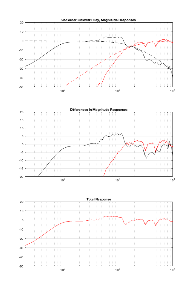
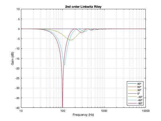
2nd order Linkwitz Reily
Figure 9.6
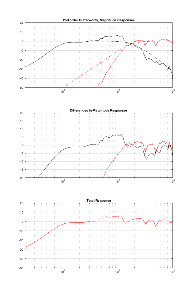
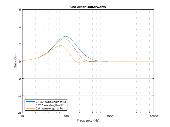
2nd order Butterworth
Figure 9.7
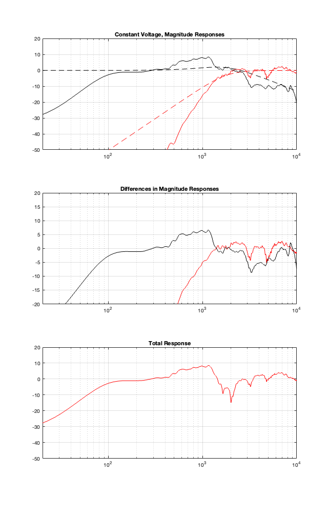
Constant Voltage
Figure 9.8
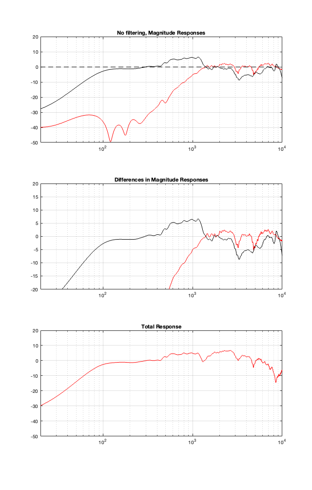
No Crossover
Figure 9.9
Comparison
Figure 9.10. The five total responses of the crossover types from the plots above.
I’ll let you draw your own conclusions about the results of these plots. I will highlight one thing: remember that the theoretical combined magnitude responses of the 4th order Linkwitz Riley and the Constant Voltage crossovers are both flat. But compare their Total Responses in the plots above. Notice that they are very different from each other. This is, in part, because the phase responses of the two signal paths are modified by the driver’s behaviours, which means that they don’t add as nicely as we would like.
The moral of the story this time is: you can’t ignore the natural response of the drivers when you’re designing your crossover. This means that we will need to change our filters to ensure that the TOTAL response of the filter PLUS the driver results in the response that we want. The design of the crossover MUST include the responses of the drivers to ensure that it behaves as we wish.
But, so far, we have only considered this at one point in space, directly in front of the loudspeaker. In the next posting, we’ll come back to looking at the total power response. Things are about to get ugly…
This will be a short posting with very little new information. I’m just starting to put some of the Lego blocks together to make it easier later on.
For this posting, I’ve taken two different pieces of information that you already have, and put them together.
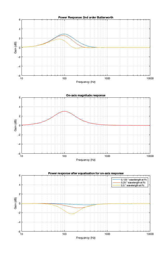
2nd order Butterworth
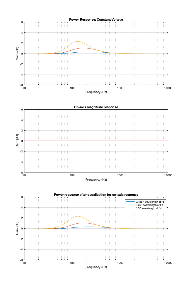
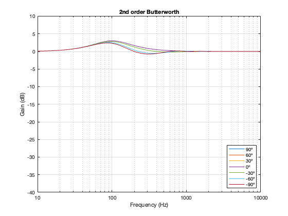
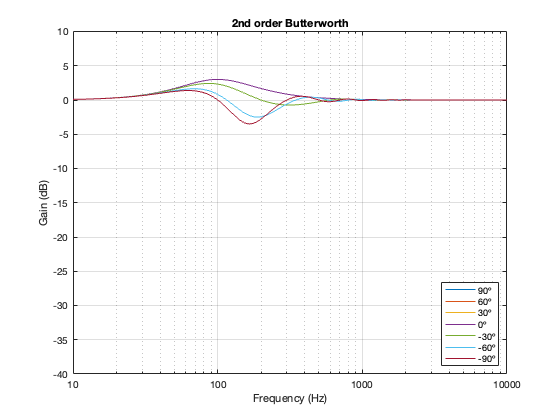
Take a look at Figure 8.1 below, which shows information related to a 2nd order Butterworth crossover at 100 Hz.
The top plot shows the power responses, explained in Part 7.
The middle plot shows the on-axis magnitude response, which will be the same regardless of the separation between the loudspeaker drivers because I’m assuming that they’re perfect point-sources.
IF you built such a loudspeaker, then chances are that you would put in an equaliser at the input of your loudspeaker to make the on-axis response flat instead of having that bump. That equaliser would, in turn effect the entire power response. So, the bottom plots show the power responses of the loudspeaker (with three different driver separations) AFTER you’ve applied the equalisation to correct for the on-axis magnitude response.
In other words, the top plots MINUS the middle red plot equals the bottom plots
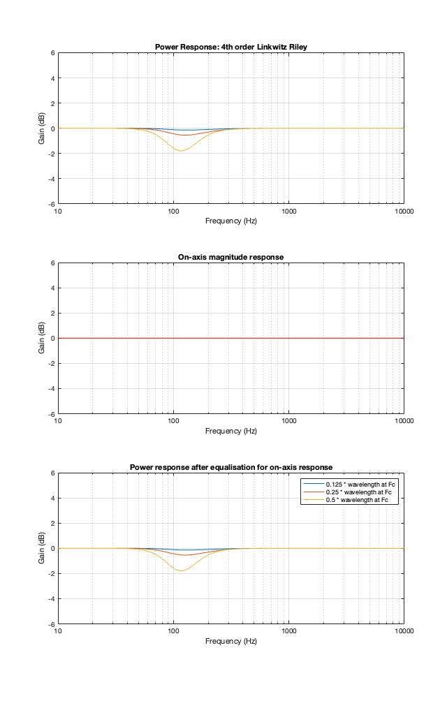
4th-order Linkwitz Riley
The 4th-order Linkwitz Riley’s power response does not change because its on-axis response is flat, so there’s nothing to correct.
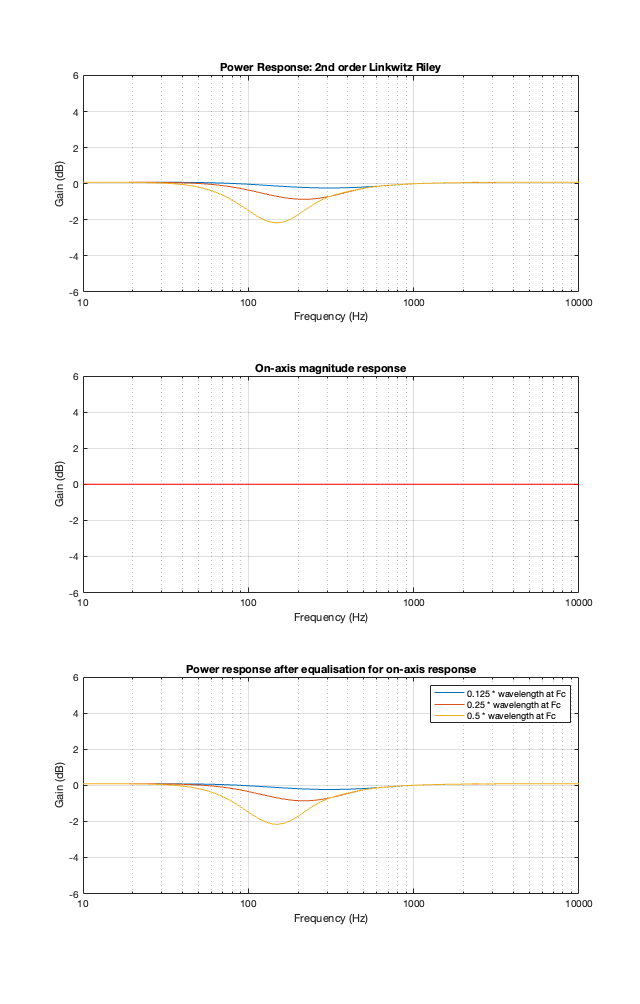
2nd-order Linkwitz Riley
The 2nd-order Linkwitz Riley’s power response does not change because its on-axis response is flat, so there’s nothing to correct.
Constant Velocity
The Constant Velocity’s power response does not change because its on-axis response is flat, so there’s nothing to correct.
Like I said: there’s no new information here. It’s just a reminder that, if you add equalisation for your on-axis response (whether this is part of your loudspeaker-building process or your installation in the listening room), you will also have a subsequent on the power response. Since the equalisation is applied to the loudspeaker’s input, the on-axis and power responses are locked together. Change one, and you change them both.
There are different ways to evaluate the behaviour of a loudspeaker. Most people like looking at the on-axis magnitude response, which is a nice and simple perspective through which one can view the universe. However, it can be VERY misleading to look at the universe from only one perspective.
As I pithily said at the end of the last posting, if you lived in an anechoic chamber and you only ever sat directly in front of your loudspeaker, then maybe you could justify being concerned only with the on-axis magnitude and phase responses of your loudspeaker. However, if you live in the real world, it’s wise to consider that some other areas of three dimensional space are also interesting – possibly even mores.
In the last posting, we moved from 0 spatial dimensions (up to Part 5, we hadn’t considered space at all…) to one dimension (I’m thinking in a geographical, or spherical view where space is defined as a horizontal and a vertical angle, and a distance, instead of X, Y, and Z coordinates. Of course, these two methods of defining space are interchangeable, if you wish to convert.) Moving vertically in that one angular dimension, we saw that the different crossover types had an effect on the directivity of the total output of the system.
Now we’ll extend to a three-dimensional world, which means that we’ll need to define space using two angles, however, don’t worry… everything will probably look familiar to you.
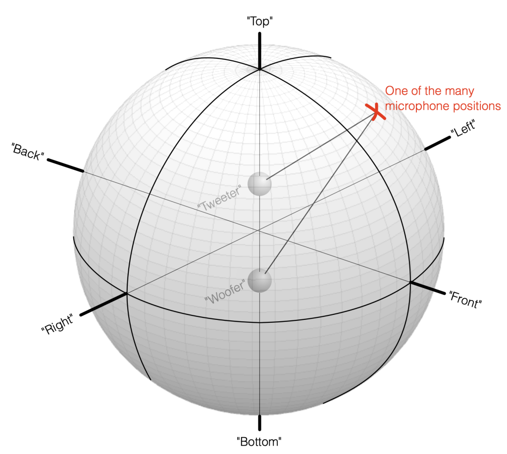
Figure 7.1: A geographic coordinate system mapped around our two point-source loudspeaker drivers
Take a look at Figure 7.1. I’ve now placed our two “perfect” omnidirectional point-source loudspeaker drivers in a three-dimensional space inside a giant sphere. I’ve called them a “tweeter” and a “woofer” again, just for the sake of clarity, but the truth is that I’m just treating them as full-range sources that are omnidirectional in all three dimensions.
We can then place our microphone at some location on the surface of that imaginary sphere, at some horizontal angle and some other vertical angle. You can consider the analysis I did in Part 6 to be a “slice” of this sphere, on the line that extends from the Bottom to the Top, running through the Front.
Sidebar Put a real loudspeaker in your living room and listen to it from out in the kitchen while you make dinner. The loudspeaker radiates sound in all directions in all three dimensions, and that spherical ball of energy is more related to what you’ll hear bleeding into the kitchen than the simple on-axis response. No one is sitting in front of the loudspeaker, so there’s no one there to care about the on-axis response at all…
Let’s move microphone around the surface of that big sphere in Figure 7.1, making a measurement of the combined outputs of the tweeter and woofer (including the delay differences caused by the distance between the two loudspeaker drivers and the three-dimensional direction to the microphone) in each place. Since the two drivers are separated in space (among other things) they’ll result in a different measurement in each location. If we then combine all of those measurements to find the total magnitude response of the three-dimensional radiation, we’ll find the total Power Response of the system. This is the combined response of the loudspeaker’s output in all three dimensions, which is what we’re looking at in this article.
There are different ways to move around that sphere and then sum the numerous measurements that you get as a result. However, if you do the math correctly, it doesn’t really matter which way to do this.
I won’t say much more here; I’ll just show the plots. Each of the Figures below has three lines on it, showing three different separations between the two loudspeaker drivers. As in the previous postings, these are 0.125, 0.25, and 0.5 * the wavelength of the crossover frequency, which, in this case is 100 Hz.
This allows you to compare the tendency of the power response characteristic as the driver separation increases.
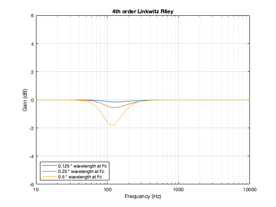
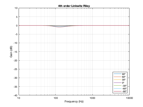
4th order Linkwitz Riley
Notice that the Power Response of the 4th-order Linkwitz Riley only drops in magnitude around the crossover frequency, and the depth and bandwidth of that dip is dependent on the distance between the drivers.
It’s also worth putting in the reminder here that if we moved the crossover to a different frequency, then the behaviour would look the same, just moved upwards or downwards on the x-axis. This is because I’m determining the distance between the two drivers using the wavelength of the crossover.
Figure 7.2
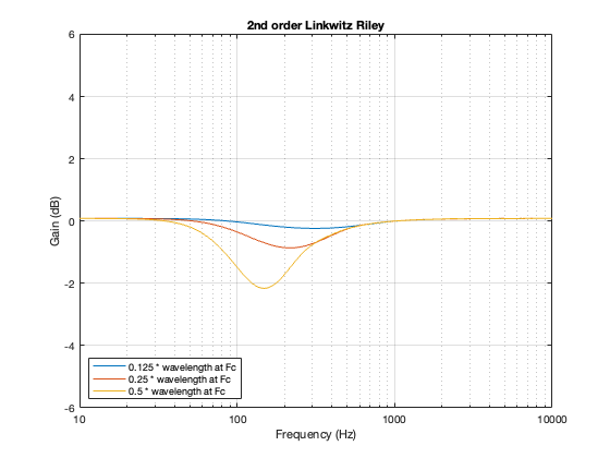
2nd order Linkwitz Riley
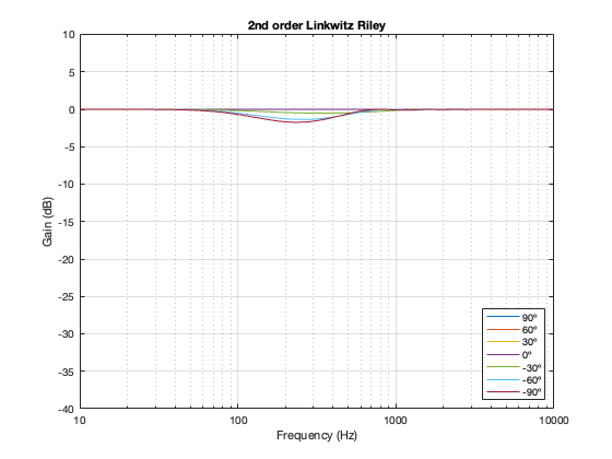
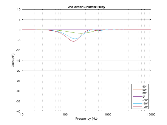
A 2nd-order Linkwitz Riley has a similar power response to the 4th order, although the effect is increased a little in frequency above the crossover, and it dips a little more for the same separation between the drivers.
Figure 7.3
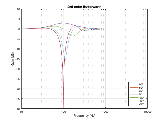
2nd order Butterworth
A 2nd-order Butterworth’s power response exhibits the opposite effect. It. produces a bump in around the crossover frequency instead of a dip. Also notice that the magnitude of the bump is more pronounced with the same distance between the loudspeaker drivers. Whereas a separation of 0.125*wavelength produced only a very slight dip in the power response for the two Linkwitz Riley crossovers, the same separation results in a more than 2 dB increase for the Butterworth design. Oddly, the bump gets smaller with larger separation – but this is a function of the relationship between the phase responses of the Butterworth filters and the delays of the two driver outputs at the various microphone positions around the sphere.
Figure 7.4
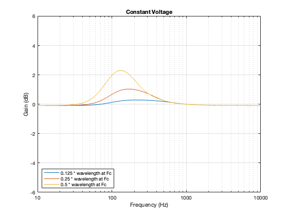
Constant Voltage
The constant voltage crossover is a little more intuitive in that the larger the separation between the drivers, the bigger the effect on the power response. In addition, it behaves similarly to the Butterworth design in that it produces a bump relative around (actually, just above) the crossover frequency.
Figure 7.5
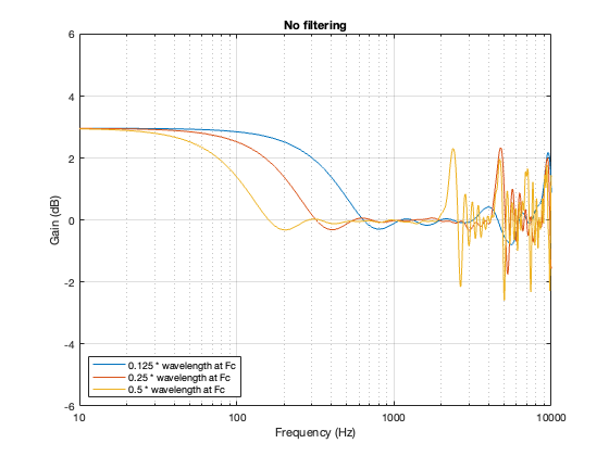
No Crossover
Again, just for curiosity’s sake, it’s interesting to look at the effect of having two drivers with the same separation as the models shown above, but without the filtering applied by a crossover. This is shown below in Figure 7.6. in the very low frequency band, you can see that the two drivers sum to give a 3 dB boost, which is equivalent to double the total power radiated by the system. The closer the two loudspeaker drivers are to each other, the higher the extension of this boost.
In addition, the strange effects in the high frequencies are essentially identical, but move up by one octave for each halving of distance between the drivers. You can also see that the interference effect is repeated each octave (notice the way that the orange and yellow lines overlap around 4 kHz, for example).
Figure 7.6
As I said in the sidebar above, if you do nothing but put in these crossover types, and your two loudspeakers are two little omnidirectional sources, then these plots will give you an idea of the difference in spectral balance that you’ll hear out in the kitchen when you play music. Of course, you would never do this. You would normally put in some extra filtering to fix things (whatever that means). In the next posting, we’ll look at what happens when you do that.
Up to now, we’ve been looking at two-way crossovers with different implementation types, analysing the responses of the two individual outputs and the total summed output as if we just mixed the two frequency bands electrically. This analysis shows us what the crossover does in isolation, but this is just a small portion of what’s happening in real life.
Let’s now start by including some real-world implications into the mix to see what happens.
For this posting, I won’t be just adding the two outputs of the high- and low-pass filter paths. We’re now going to pretend that the outputs of those two paths are connected to two point-source loudspeakers floating in infinite space. Since they’re both point sources, each one has a flat magnitude response and a flat phase response relative to its input, and these two characteristics are true in all directions. They also have no frequency limits. So, although I’m calling one a “tweeter” and the other a “woofer”, they don’t behave like real loudspeakers.
Using this kind of model allows me to analyse the implications of the differences in distances to the microphone (or listening) position, including the characteristics of the crossover.
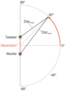
Figure 6.1.
Figure 6.1 shows a schematic diagram of the system that we’re analysing in this posting. As you ca see, the “tweeter” and “woofer” are separated by some vertical distance. The microphone position is at some distance from the centre of the two loudspeakers (the radius of the big semi-circle in the drawing), and at some angle above or below the on-axis angle to the loudspeaker pair. In my analyses, negative angles are below the horizon, and positive angles are above.
If the angle is 0º, then the distances to the tweeter and the woofer are identical, and the result is the same as the plots I’ve shown in Parts 2, 3, 4, and 5. However, if the angle to the microphone goes positive, then this means that the woofer’s signal will be delayed relative to the tweeter’s, and this will have some effect on the way the two signals interfere with each other when they are summed.
This change in interference results in a change in the magnitude response of the summed signals at the microphone as a function of the angle. So, another way to consider this is that we’re changing the directivity of the loudspeaker pair.
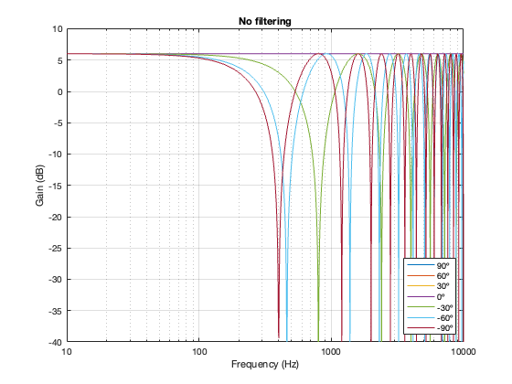
For all of the plots below, I’ve shown the responses at angles in 30º increments from -90º to 90º. As I’ve said above, the 0º plot should be identical to the plot for the same crossover type shown in one of the previous postings.
Of course, a change in the separation between the two drivers will change the amount of effect on the magnitude response when the angle to the microphone is not 0º. For these plots, I’ve decided to keep the crossover frequency at 100 Hz, to maintain consistency, and to plot the responses for 3 example loudspeaker separations: 43.125 cm (0.125 * wavelength at 100 Hz), 86.25 cm (0.25 * wavelength at 100 Hz), and 1.725 m (0.5 * wavelength at 100 Hz).
The point of these is not really to give “real world” suggestions, but to show tendencies…
Not surprisingly, the greater the separation between the loudspeaker drivers, the bigger the effect on the magnitude response off-axis. Notice, however, that the effect is not symmetrical. In other words, the magnitude responses at -90º and 90º are not the same. This is because the relative phase responses of the two filter paths (also remembering that the tweeter’s signal is flipped in polarity) has an effect on the sum of the two signals at different points in space.
Hopefully, it’s clear that if the crossover had been at a different frequency, the characteristics of the magnitude responses would have been the same – they would have just moved in frequency. This is because I’m relating the separation between the two loudspeaker drivers as a fraction of the wavelength of the crossover frequency.
And, of course, you don’t need to email me to remind me that a loudspeaker separation of 1.725 m is silly. As I said, the point of this is NOT to help you design a loudspeaker, it’s to show the characteristics and the tendencies. (On the other hand, 1.725 m between a subwoofer and a main loudspeaker is not silly… so there…)
Notice here that the magnitude responses never go above 0 dB at any angle. It’s also interesting that at smaller separations, the difference in the magnitude response as a function of angle is smaller than that for the 2nd-order Butterworth crossover.
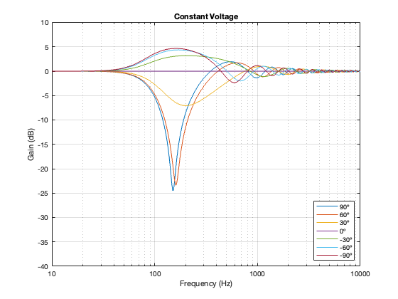
As I mentioned in the previous posting, there are many ways to implement a constant voltage crossover. The plots below show analyses of the same crossover as the one I shows in Part 5 – using a 2nd-order Butterworth for the high-pass section, and subtracting that from the input to create the low-pass section.
Figure 6.11. 100 Hz, Constant Voltage Separation = 0.125 * wavelength at 100 Hz
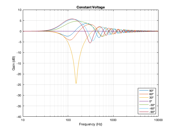
Figure 6.12. 100 Hz, Constant Voltage Separation = 0.25 * wavelength at 100 Hz
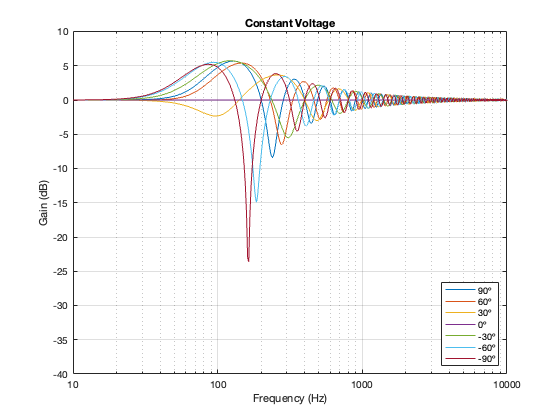
Figure 6.13. 100 Hz, Constant Voltage Separation = 0.5 * wavelength at 100 Hz
One thing to notice here is that, although we saw in Part 5 that a constant voltage crossover’s output is identical to its input, that’s only true for the hypothetical example where we just summed the outputs. You’ll notice that, at a microphone angle of 0º in this still-hypothetical example, the total magnitude response is still flat. However, at other angles, the change in magnitude response is much larger than it is for the other crossover types for angles between -60º and 60º. Therefore, if you jumped to the conclusion in the previous posting that a constant voltage design is the winner, you might want to re-consider if you don’t live in a room that extends to infinite space without any walls (or a perfect anechoic chamber), and you only listen on-axis to the loudspeaker.
Just sayin’…
P.S.
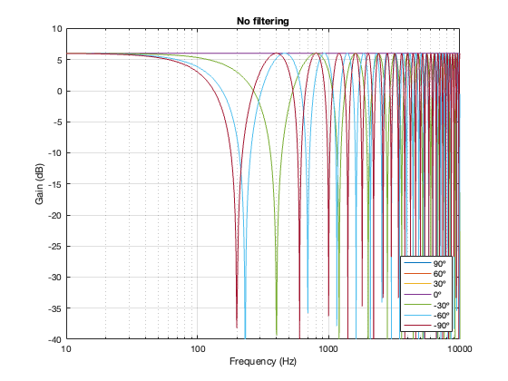
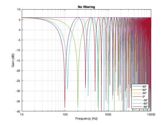
In case you’re wondering, it’s also possible to look at the effects of summing the outputs of the two loudspeakers without including a crossover in the signal path. The result of this is that you have two full-range drivers, whose only difference at the microphone position is the time of arrival as a function of the angle of the microphone relative to the “horizon”. This results in two big differences in what you see above:
The total output when the interference is construction is + 6 dB relative to the input. This happens because the two signals are identical, and, at some frequencies and some microphone positions, they just add together.
The interference extends to a much wider frequency band, since both loudspeakers’ signals are interfering with each other at all frequencies.
Figure 6.14. No crossover Separation = 0.125 * wavelength at 100 Hz
Figure 6.16. No crossover Separation = 0.5 * wavelength at 100 Hz
The four crossover types we’ve looked at so far all use the same basic concept: take the input signal and divide it into different frequency bands using some kind of filters that are implemented in parallel. You send the input to a high pass filter to create the high-frequency output, and you send the same input to a low-pass filter to create the low-frequency output.
In all of the examples we’ve seen so far, because they have been based on Butterworth sections, incur some kind of phase shift with frequency. We’ll talk about this more later. However, the fact that this phase shift exists bothers some people.
There are various ways to make a crossover that, when you sum its outputs, result in a total that is NOT phase shifted relative to the input signal. The general term for this kind of design is a “Constant Voltage” crossover (see this AES paper by Richard Small for a good discussion about constant voltage crossover design).
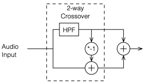
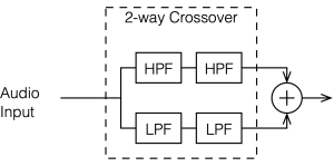
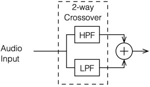
Let’s look at just one example of a constant voltage crossover to see how it might be different from the ones we’ve looked at so far. To create this particular example, I take the input signal and filter it using a 2nd-order Butterworth high pass. This is the high-frequency output of the crossover. To create the low-frequency output of the crossover, I subtract the high-frequency output from the input signal. This is shown in the block diagram below in Figure 5.1
Figure 5.1. One example of a constant voltage crossover.
As with the previous four crossovers, I’ve added the two outputs of the crossover back together to look at the total result.
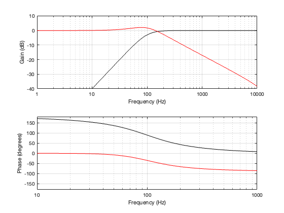
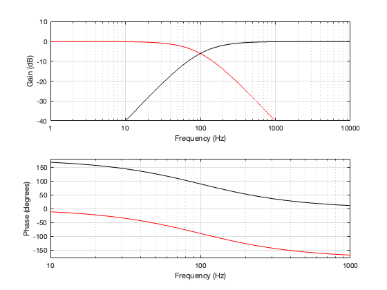
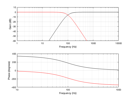
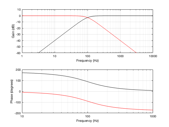
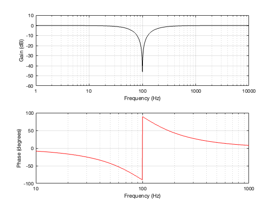
Figure 5.2: the magnitude and phase responses of the two sections of the crossover.
Figure 5.2 shows the magnitude and phase responses of the high- and low-frequency portions of the crossover. One thing that’s immediately noticeable there is that the two portions are not symmetrical as they have been in the previous crossover types. The slopes of the filters don’t match, the low-pass component has a bump that goes above 0 dB before it starts dropping, and their phase responses do not have a constant difference independent of frequency. They’re about 180º apart in the low end, and only about 90º in the high end.
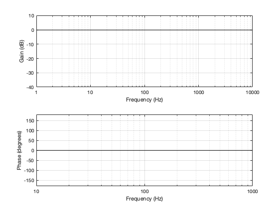
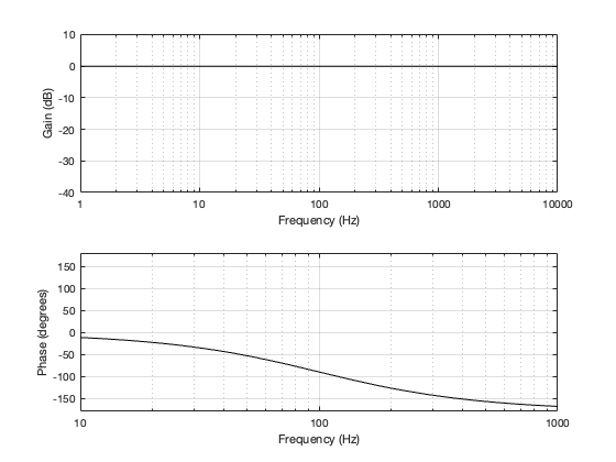
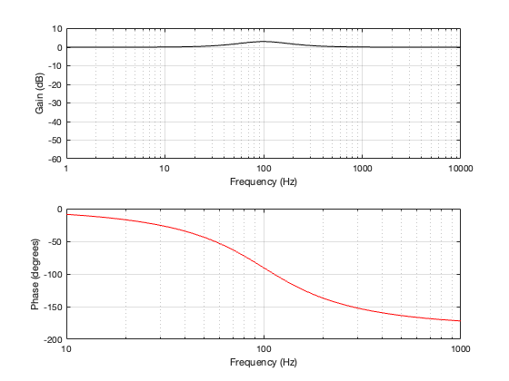
However, because the low-frequency output was created by subtracting the high-frequency component from the input, when we add them back together, we just get back what we put in, as can be seen in Figure 5.3.
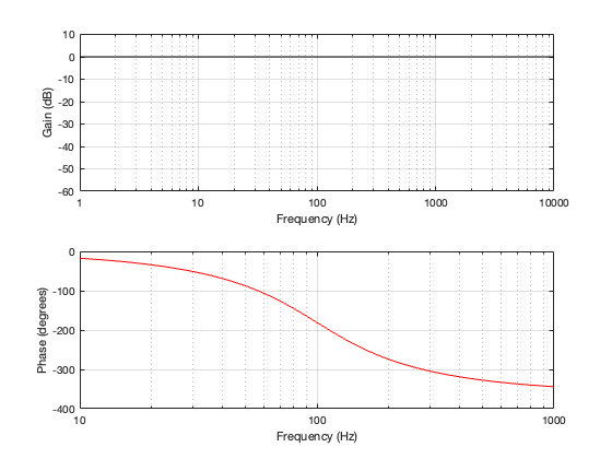
Figure 5.3. The magnitude and phase responses of the summed output of the crossover shown in Figure 5.1.
Essentially, this shows us that Output = Input, which is hopefully, not surprising.
If we then run our three sinusoidal signals through this crossover and look at the summed output, the results will look like Figures 5.4 to 5.6
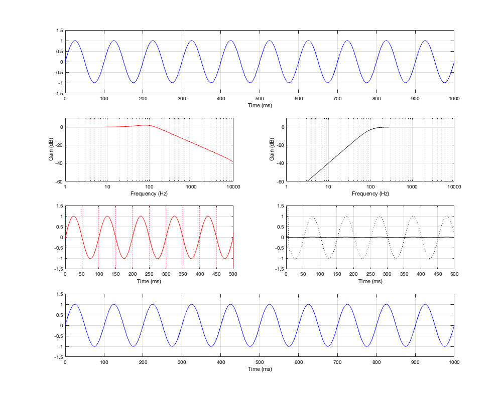
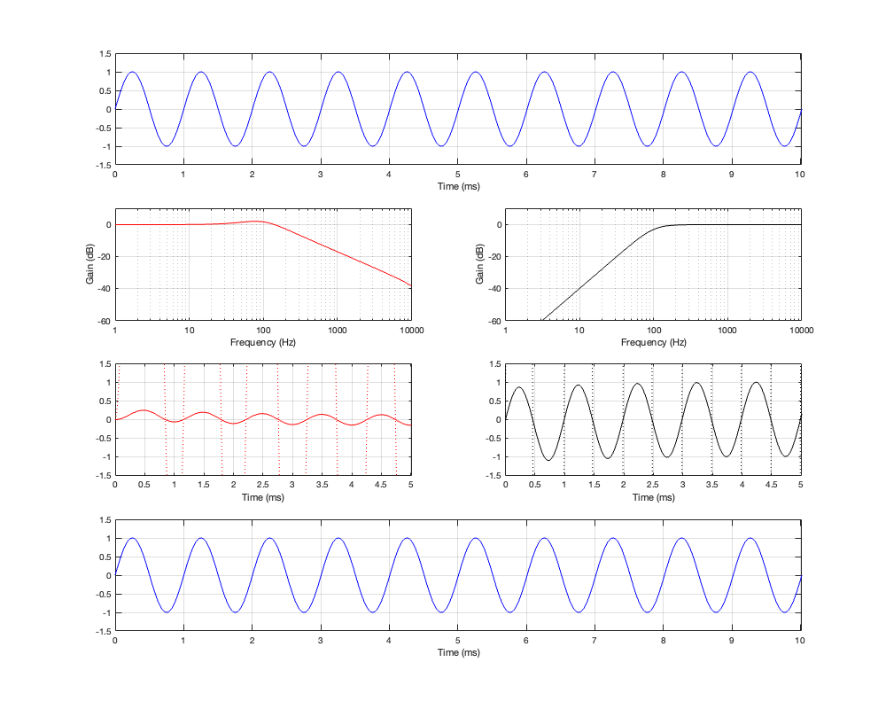
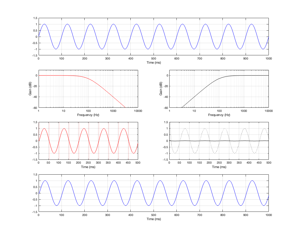
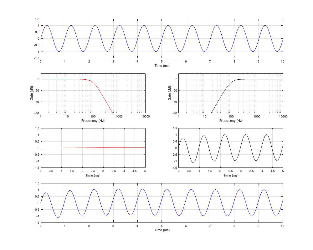
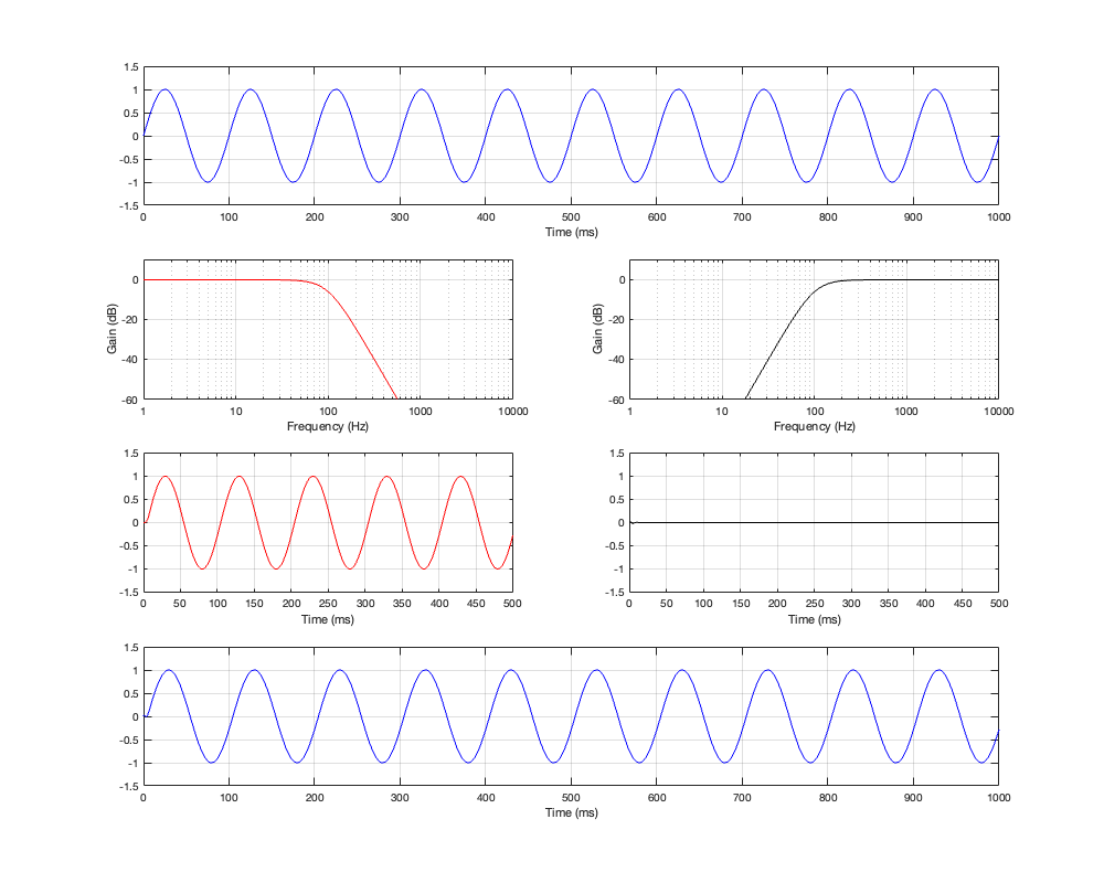
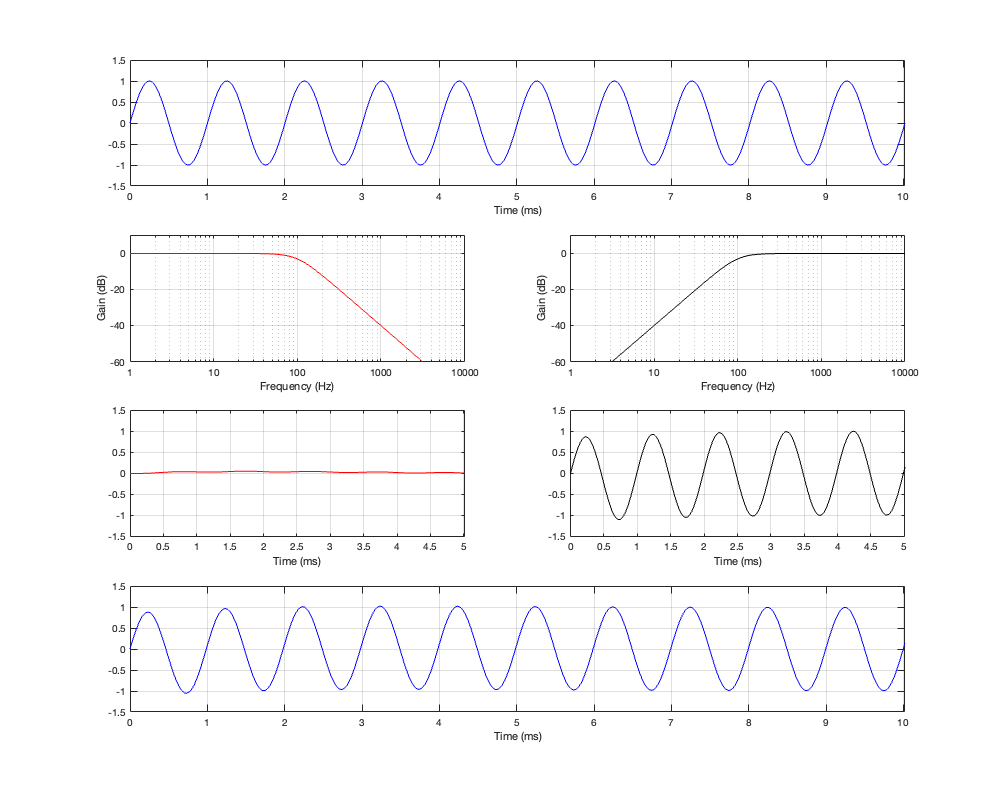
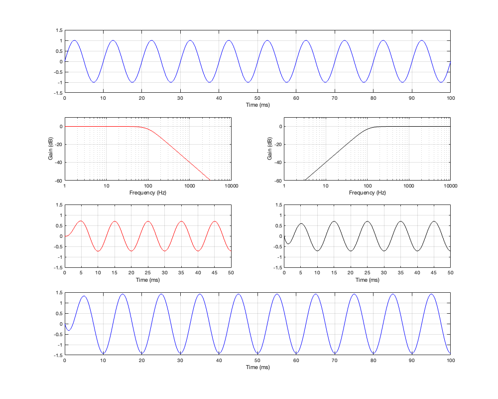
Figure 5.4: Row 1: the input (10 Hz sine wave). Row 2: the magnitude responses of the two filters. Row 3: the outputs of the individual filters. Row 4: the summed output
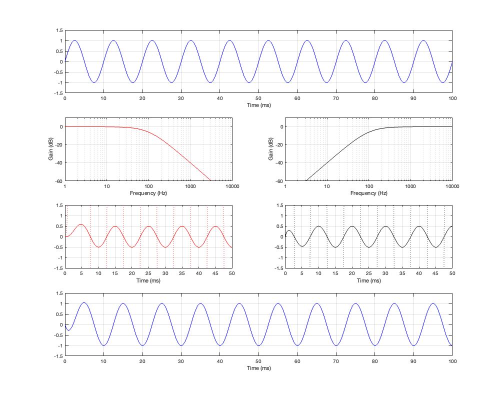
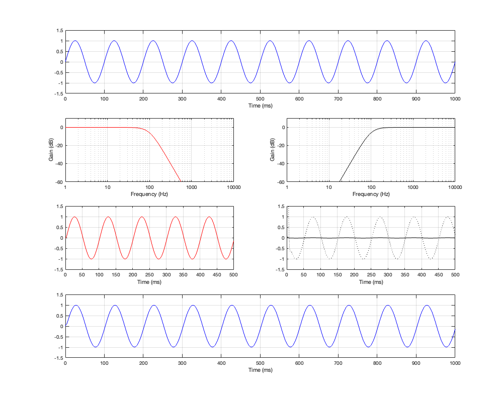
Figure 5.5: Row 1: the input (100 Hz sine wave). Row 2: the magnitude responses of the two filters. Row 3: the outputs of the individual filters. Row 4: the summed output
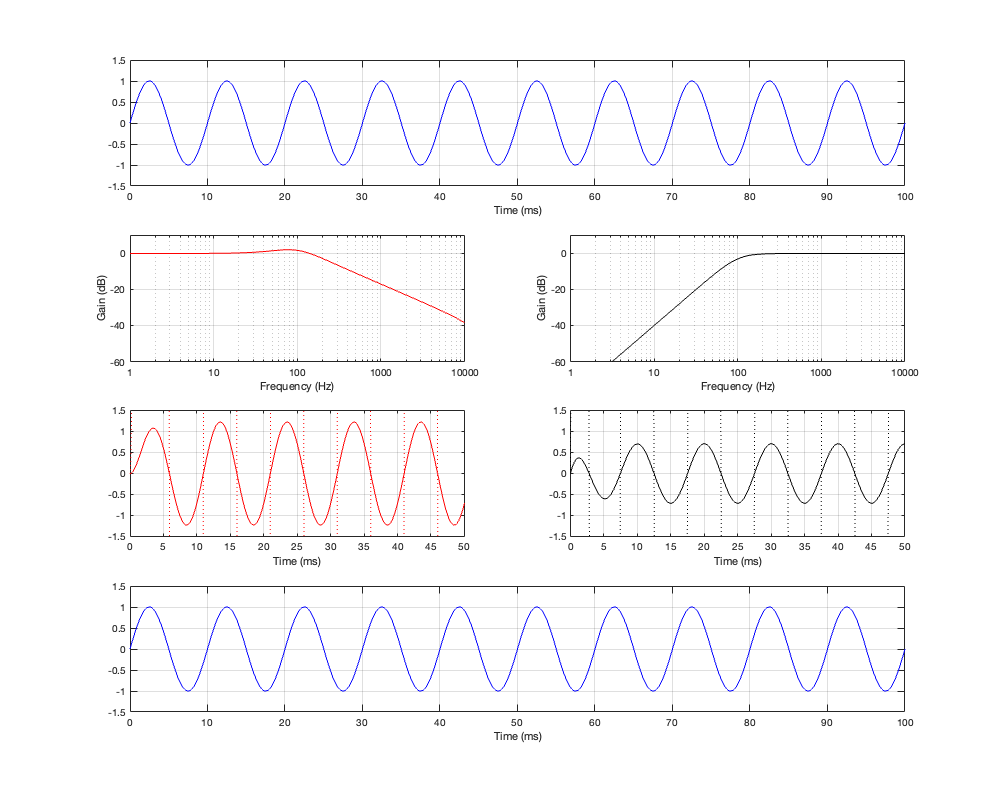
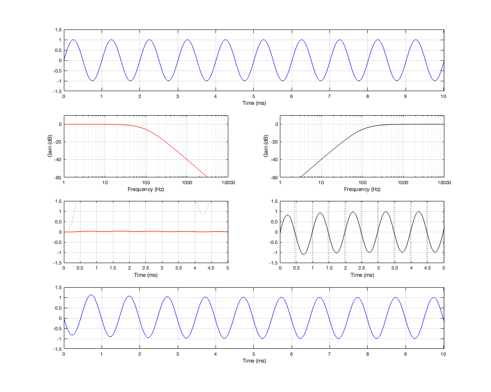
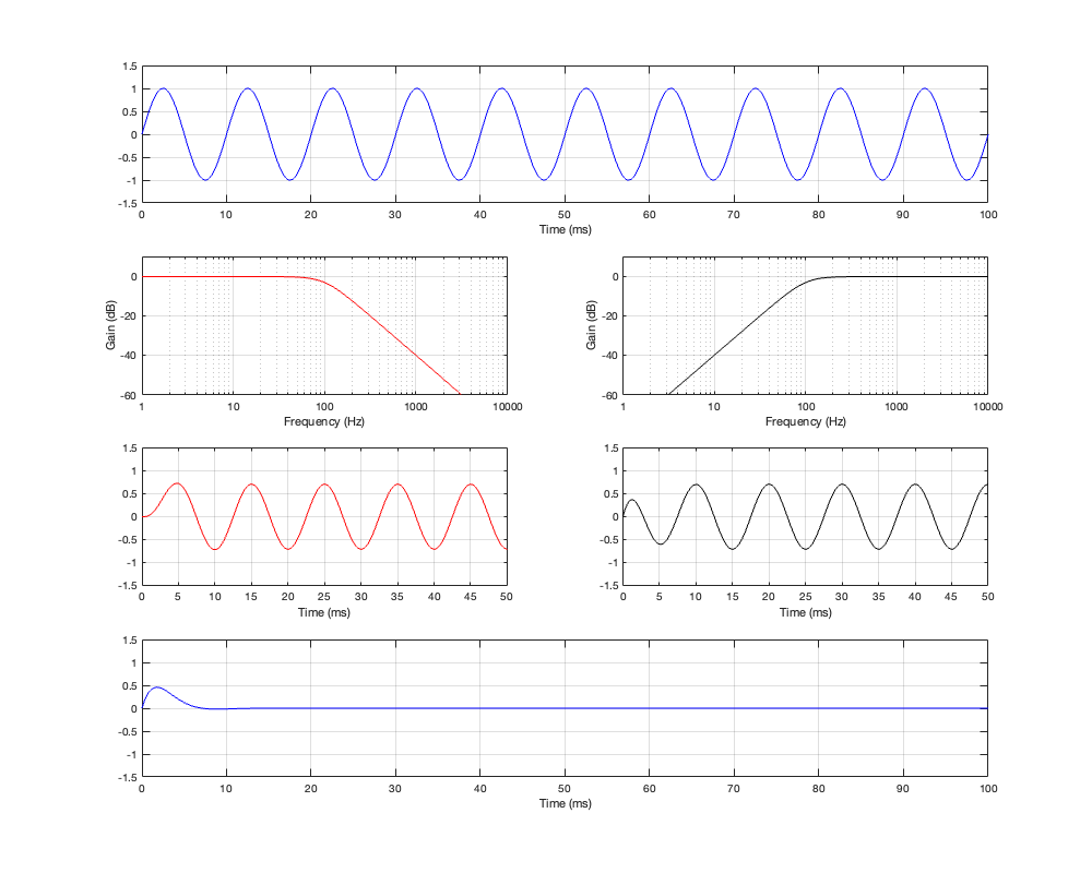
Figure 5.6: Row 1: the input (1 kHz sine wave). Row 2: the magnitude responses of the two filters. Row 3: the outputs of the individual filters. Row 4: the summed output
Notice in all three of those figures that the outputs and the inputs are identical, even though the individual behaviours of the two frequency-limited outputs might be temporarily weird (look at the start of the signals of the high-frequency output in Figures 5.4 and 5.6 for example…)
Now, don’t go jumping to conclusions… Just because the sum of the output is identical to the input of a constant voltage crossover does NOT make this the winner. We’re just getting started, and so far, we have only considered a very simple aspect of crossovers that, although necessary to understand them, is just the beginning of considering what they do in the real world.
Up to now, we have really only been thinking about crossovers in three dimensions: Frequency, Magnitude, and Phase. Starting in the next posting, we’ll add three more dimensions (X,Y, and Z of physical space) to see how, even a simple version of the real world makes things a lot more complicated.
A 2nd-order Linkwitz Riley crossover is something like a hybrid of the previous two crossover types that I’ve described. If you’re building one, then the “helicopter view” block diagram looks just like the one for the 4th-order Linkwitz Riley, but I’ve shown it here again anyway.
Figure 4.1
The difference between a 2nd-order and a 4th-order Linkwitz Riley is in the details of exactly what’s inside those blocks called “HPF” and “LPF”. In the case of a 2nd-order crossover, each block contains a 1st-order Butterworth filter, and they all have the same cutoff frequency. (For a 4th-order Linkwitz Riley, the filters are all 2nd-order Butterworth)
Since each of those filters will attenuate the signal by 3 dB at the cutoff frequency, then the total combined response for each section will be -6 dB at the crossover. This can be seen below in Figure 4.2. Also, the series combination of the two 1st-order Butterworths means that the high and low sections of the crossover will have a phase different of 180º at all frequencies.
Figure 4.2
Since the two filter sections have a phase separation of 180º, we need to invert the polarity of the high-pass section. This means that, when the two outputs are summed as shown in Figure 4.1, the total magnitude response is flat, but the phase response is the same as a 2nd-order minimum phase allpass filter, as can be seen in Figure 4.3, below.
Figure 4.3
If we then look at the low- mid- and high-frequency sinusoidal signals that have been passed through the crossover, the results look like those shown below in Figures 4.4, 4.5, and 4.6.
Figure 4.4: Row 1: the input (10 Hz sine wave). Row 2: the magnitude responses of the two filters. Row 3: the outputs of the individual filters. Row 4: the summed output
As can be seen in Figure 4.4, for a very low frequency, the output is the same as the input, the magnitude is identical (as we would expect based on the Magnitude Response plot shown in Figure 4.3, and the phase difference of the output relative to the input is 0º.
Figure 4.5: Row 1: the input (100 Hz sine wave). Row 2: the magnitude responses of the two filters. Row 3: the outputs of the individual filters. Row 4: the summed output
At the crossover frequency, shown in Figure 4.5, the output has shifted in phase relative to the input by 90º, but their magnitudes still match.
Figure 4.6: Row 1: the input (1 kHz sine wave). Row 2: the magnitude responses of the two filters. Row 3: the outputs of the individual filters. Row 4: the summed output
At a high frequency, the phase has shifted by 180º relative to the input.
One last thing. The dotted plots in Figures 4.4 to 4.6 are the signals magnified by a factor of 10 to make them easier to see when they’re low in level. There are two interesting ones to look at:
the very beginning of the black plot on the right of Figure 4.4. Notice that this one starts with a positive spike before it settles down into a sinusoid.
the red plot on the left In Figure 4.6. Notice that the signal goes positive, and stays positive for the full 5 ms.
We will come back later to talk about both of these points. The truth is that they’re not really important for now, so we’ll pretend that they didn’t look too weird.
A fourth-order Linkwitz-Riley crossover is made using the same filters in the 2nd-order Butterworth crossover described in the previous posting. The difference in implementation is that you use two second-order filters in series. Again, all filters have the same cutoff frequency and, if you’re implementing them with biquads, the Q of all of them is 1/sqrt(2).
Figure 3.1
Since we have two high pass filters in series, then the total result is -6 dB at the cutoff frequency (since each of the two filters attenuates by 3 dB) and the slope of the filter is 24 dB per octave. This results in the magnitude and phase responses shown below in Figure 3.2.
Figure 3.2
One important thing to notice now is that the phase responses of the two filters are 360º apart at all frequencies. This is different from the second-order Butterworth crossover, in which the two outputs are 180º apart. So we won’t need to flip the polarity of anything to compensate for the phase difference.
As in the previous posting, Let’s look at the signals that get through the crossover, and the total summed output for three input frequencies. This is shown in Figure 3.3, 3.4, and 3.5.
Figure 3.3: Row 1: the input (1 kHz sine wave). Row 2: the magnitude responses of the two filters. Row 3: the outputs of the individual filters. Row 4: the summed output
Figure 3.4: Row 1: the input (10 Hz sine wave). Row 2: the magnitude responses of the two filters. Row 3: the outputs of the individual filters. Row 4: the summed output
Figure 3.5: Row 1: the input (100 Hz sine wave). Row 2: the magnitude responses of the two filters. Row 3: the outputs of the individual filters. Row 4: the summed output
If you take a look at Figures 3.3 and 3.4 it appears that the total summed output of the crossover is in phase with the input at very low and very high frequencies. However, this is actually misleading. Take a look at Figure 3.5 and you’ll see that, when the input signal is the same frequency as the crossover frequency, the summed output is shifted by 180º relative to the input signal.
Figure 3.6
If we compare the summed output to the input, they are in-phase at very low frequencies. As the frequency increases, the phase of the summed output of the crossover gets later and later, passing 180º at the crossover frequency and approaching a shift of 360º in the high frequencies.
In other words, a 4th-order Linkwitz-Riley crossover by itself, when you sum the outputs of the filters as shown in Figure 3.1, has the same response as a 4th-order minimum phase allpass filter.
One extra thing to notice is that, since the high-pass and low-pass paths are 360º apart, and (partly) since they’re -6 dB at the crossover frequency, the magnitude response of the summed total is flat.
One way to look at the behaviour of a signal when it’s sent through a crossover is to pretend that the loudspeaker isn’t part of the system. Once-upon-a-time, I probably would have phrased this differently and said something like “pretend that the loudspeaker is perfect”, but, now that I’m older, my opinions about the definition of “perfect” have changed.
So, we’ll take a signal, send it to a two-way crossover of some kind, and then just add the two signals back together. This shows us one view of the behaviour of the crossover, which is good enough to deal with the basics for now. In a later posting in this series, we’ll look at a more multi-dimensional and therefore realistic view of what’s happening.
Figure 2.1
The block diagram above shows the signal flow that I used for all of the following plots in this posting.
Butterworth, 2nd-order (12 db/octave)
Although the block diagram above shows that we have a high-pass and a low-pass filter to separate the signal into two frequency bands, there are a lot of details missing about the specific characteristics of those filters. There are many ways to make a high-pass filter, for example…
One common crossover type uses 2nd-order Butterworth filters, both with the same cutoff frequency. One way to implement these are to use biquads to make low-pass and high-pass filters with Q = 1/sqrt(2).
Fig. 2.2: The individual magnitude and phase responses of the low-pass (in red) and high-pass (in black)
Before we look at the output of the entire crossover after the two signals have been summed, let’s talk about the red and the black curves in the plots above.
The magnitude responses should not come as a surprise. The fact that I’m using 2nd-order filters means that the slope of the attenuation will be 12 dB per octave (or 40 dB per decade) once you get far enough away from the cutoff frequency. The fact that they also have a Q of 1/sqrt(2) (approximately 0.707) means that they will attenuate the signal by 3 dB at the cutoff frequency, and that there is no “bump” in the slope of the magnitude response.
However, the phase responses might be a little confusing. Let’s take those separately:
For the low-pass filter (the black line), you can see that in the high-frequency band, where the magnitude response is a flat line at 0 dB (which means that the level of the output level is equal to the level of the input), the phase shift is 0º.
Another way to look at this is to put a sine wave into the system and see what comes out, as shown in Figure 2.3 below. The top plot shows the input to the two filters. Since this sine wave has a period of 1 ms, then it’s a 1000 Hz tone.
The second row of plots shows the magnitude responses of the low-pass filter (in red, on the left) and the high-pass filter (in black, on the right). Notice the levels of these two curves at a frequency of 1000 Hz.
The third row of plots shows the actual outputs of the two filters. For now, we’ll only look at the output of the high-pass filter on the right. There are three things to notice about this plot:
After about 1 ms, the amplitude of this sine tone is the same as the one in the top plot.
The phase of this sine tone is the same as the one in the top plot. In other words (for example), they both pass the 0 line, heading positive at Time = 1 ms.
The start of the sine wave is a little weird. Notice that the positive peak is lower than expected and first negative trough is BELOW the maximum-negative amplitude. (it’s below a value of -1). We’ll ignore this for now, and come back to it later.
The fourth row shows the output of the two filters when they have been added together. Notice here that the output is almost identical to the input because it’s essentially just the contribution of the high-pass filter. The low-pass filter has so little output that it’s practically irrelevant.
Figure 2.3: Row 1: the input (1 kHz sine wave). Row 2: the magnitude responses of the two filters. Row 3: the outputs of the individual filters. Row 4: the summed output
Let’s now look a what happens if we put in a low-frequency sine wave instead. This is shown in Figure 2.4.
Figure 2.4 Row 1: the input (10 Hz sine wave). Row 2: the magnitude responses of the two filters. Row 3: the outputs of the individual filters. (the dotted line shows the signal with its amplitude multiplied by 10 to “zoom in” on it) Row 4: the summed output
Notice now that the time scale is 100 times longer. The sine wave now has a period of 100 ms, so it’s a 10 Hz sine wave.
We’ll focus on the third row of plots again, still looking only at the output of the high-pass filter on the right. There are three things to notice about this plot:
After about 100 ms, the amplitude of this sine tone (the solid black line) is MUCH lower than the amplitude of the input. The dotted line is a “magnified” version of the same signal so that we can see it for the phase comparison.
The phase of this sine tone is the shifted by 180º relative to the top plot. In other words (for example), at Time = 200 ms they both pass the 0 line, but this signal is going negative when the input is going positive.
The start of the sine wave is a also weird, but differently so; with that spike at the beginning and the weird wiggle in the curve before it settles down. We’ll ignore this for now, and come back to it later.
If you go back and look at the low-pass filter’s output, then you’ll see basically the same behaviour, but for the opposite frequency.
And, again, the output is almost identical to the input because it’s essentially just the contribution of the low-pass filter. The high-pass filter has so little output that it’s practically irrelevant.
Now let’s look at what happens when the frequency of the input signal is on the cutoff frequency of the two filters – in other words, the crossover frequency.
Figure 2.5: Row 1: the input (100 Hz sine wave). Row 2: the magnitude responses of the two filters. Row 3: the outputs of the individual filters. Row 4: the summed output
Now the sine wave has a period of 10 ms, so its frequency is 100 Hz.
Take a look at the third row of plots at Time = 10 ms.
The first thing to do is to compare the outputs of the two filters. The output of the low-pass filter on the left is negative, whereas the output of the high-pass filter on the right is positive. The outputs of the two filters are 180º out of phase with each other. This can also be seen in the plot back in Figure 2.2, where it’s shown that the difference between the red and the black phase response plots is 180º at all frequencies.
This is also why., once everything settles down, the sum of the two filters (the blue line on the bottom) is silence. The two signals have equal amplitude, and are 180º out of phase, so they cancel each other out.
Now compare those signal plots in the third row in Figure 2.5 to the input signal shown in the top plot. If you look at Time = 10 ms again (for example), you can see that the output of the low-pass filter is 90º behind the input. However, the output of the high-pass filter is early 90º ahead of the input.
The fact that the phase of the output of the high-pass filter is ahead of its own input confuses many people, however, don’t panic. This does not mean that the output is ahead of the input in TIME. The high-pass filter cannot see into the future. The only reason its output can have a phase that precedes the phase of its input is if the sine wave has been playing for a long time (and, in this case a “long” time can be measured in milliseconds…).
This confusion is the result of two things:
People are typically taught the concept of phase as it relates to time. However, if you’re talking about a sine wave, then you are implying infinite time. in order for a signal to be a REAL sine wave, it must have always been playing and it must never stop. If it started or stopped, then there are other frequencies present, and so it’s not a theoretically-perfect sine wave.
We use the words “ahead” and “behind” or “earlier” and “later” to describe the phase relationships, and these words typically imply a time relationship.
Maybe a rough analogy that can help is to walk next to a friend, at the same speed, but do not synchronise your steps. You will both arrive at the same place at the same time, but at two different moments in the cycles of your footsteps.
Of course, if you make a crossover like this, it won’t work very well, since you get that cancellation at the crossover frequency when the two filters outputs are added together. If we plot the summed response’s magnitude and phase characteristics, they look like the plots shown in Figure 2.6.
Figure 2.6: the magnitude and phase responses of the total shown in Figure 2.5.
As you can see there, there is complete cancellation at the crossover frequency, and the phase response flips across that notch.
So, the solution with a 2nd-order Butterworth crossover is to assume that people won’t notice if you invert the polarity of the high-pass filter’s output. This is a good assumption that I will not argue with at all.
This polarity inversion “undoes” the 180º phase difference of the two filters seen in Figure 2.2, and the summed result is shown below in Figure 2.7 and 2.8.
Figure 2.7: the magnitude and phase responses of the total shown in Figure 2.8, which is the same as Figure 2.5 after the polarity of the HPF’s output has been inverted.
Figure 2.8: Row 1: the input (100 Hz sine wave). Row 2: the magnitude responses of the two filters. Row 3: the outputs of the individual filters. (Note that the polarity of the HPF’s output has been inverted) Row 4: the summed output
Now the outputs of the two filters appear to be in phase with each other. They are still 90º out of phase with the input, which means that their summed outputs are also 90º out of phase with the input. This can be seen in the bottom plots of Figure 2.7 and 2.8.
You’ll also notice that there is a 3 dB bump at the crossover frequency. This is because, at their cutoff frequencies, both filters attenuate by 3 dB (a linear gain of 0.707). When those two signals of equal amplitude and matching phase are added together, you get a magnitude that is 6 dB higher (or a linear gain of 1.41). We’ll talk about this later when we start looking at the real world.
Finally, take a look at the bottom plot in Figure 2.7. You can see there that the summed outputs of the two filters result in a phase shift that increases with frequency. In fact, when we look at a 2nd-order Butterworth crossover like this, without all the real-world implications of loudspeaker drivers that have their own characteristics and are separated in space, it can be seen that it acts as a 2nd-order minimum-phase allpass filter. This isn’t necessarily a bad thing, so don’t jump to conclusions this early…
We are STILL not going to talk about that weirdness at the beginning of the signal after it’s been filtered. That will come later.
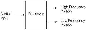
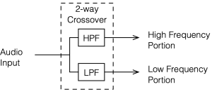
A crossover is a set of filters that take an audio signal and separate it into different frequency portions or “bands”.
For example, possibly the simplest type of crossover will accept an audio signal at its input, and divide it into the high frequency and the low frequency components, and output those two signals separately. In this simple case, the filtering would be done with
a high-pass filter (which allows the high frequency bands to pass through and increasingly attenuates the signal level as you go lower in frequency), and
a low-pass filter (which allows the low frequency bands to pass through and increasingly attenuates the signal level as you go higher in frequency).
This would be called a “Two-way crossover” since it has two outputs.
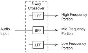
Crossovers with more outputs (e.g. Three- or Four-way crossovers) are also common. These would probably use one or more band-pass filters to separate the mid-band frequencies.
Why do we need crossovers?
In order to understand why we might need a crossover in a loudspeaker, we need to talk about loudspeaker drivers, what they do well, and what they do poorly.
It’s nice to think of a loudspeaker driver like a woofer or a tweeter as a rigid piston that moves in and out of an enclosure, pushing and pulling air particles to make pressure waves that radiate outwards into the listening room. In many aspects, this simplified model works well, but it leaves out a lot of important information that can’t be ignored. If we could ignore the details, then we could just send the entire frequency range into a single loudspeaker driver and not worry about it. However, reality has a habit of making things difficult.
For example, the moving parts of a loudspeaker driver have a mass that is dependent on how big it is and what it’s made of. The loudspeaker’s motor (probably a coil of wire living inside a magnetic field) does the work of pushing and pulling that mass back and forth. However, if the frequency that you’re trying to produce is very high, then you’re trying to move that mass very quickly, and inertia will work against you. In fact, if you try to move a heavy driver (like a woofer) a lot at a very high frequency, you will probably wind up just burning out the motor (which means that you’ve melted the wire in the coil) because it’s working so hard.
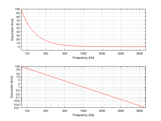
Another problem is that of loudspeaker excursion, how far it moves in and out in order to make sound. Although it’s not commonly known, the acoustic output level of a loudspeaker driver is proportional to its acceleration (which is a measure of its change in velocity over time, which are dependent on its excursion and the frequency it’s producing). The short version of this relationship is that, if you want to maintain the same output level, and you double the frequency, the driver’s excursion should reduce to 1/4. In other words, if you’re playing a signal at 1000 Hz, and the driver is moving in and out by ±1 mm, if you change to 2000 Hz, the driver should move in and out by ±0.25 mm. Conversely, if you halve the frequency to 500 Hz, you have to move the driver in and out with an excursion of ±4 mm. If you go to 1/10 of the frequency, the excursion has to be 100x the original value. For normal loudspeakers, this kind of range of movement is impractical, if not impossible.
Note that both of these plots show the same thing. The only difference is the scaling of the Y-axis.
One last example is that of directivity. The width of the beam of sound that is radiated by a loudspeaker driver is heavily dependent on the relationship between its size (assuming that it’s a circular driver, then its diameter) and the wavelength (in air) of the signal that it’s producing. If the wavelength of the signal is big compared to the diameter of the driver, then the sound will be radiated roughly equally in all directions. However, if the wavelength of the signal is similar to the diameter of the driver, then it will emit more of a “beam” of sound that is increasingly narrow as the frequency increases.
So, if you want to keep from melting your loudspeaker driver’s voice coil you’ll have to increasingly attenuate its input level at higher frequencies. If you want to avoid trying to push and pull your tweeter too far in and out, you’ll have to increasingly attenuate its input level at lower frequencies. And if you’re worried about the directivity of your loudspeaker, you’ll have to use more than one loudspeaker driver and divide up the signal into different frequency bands for the various outputs.