Power Response
There are different ways to evaluate the behaviour of a loudspeaker. Most people like looking at the on-axis magnitude response, which is a nice and simple perspective through which one can view the universe. However, it can be VERY misleading to look at the universe from only one perspective.
As I pithily said at the end of the last posting, if you lived in an anechoic chamber and you only ever sat directly in front of your loudspeaker, then maybe you could justify being concerned only with the on-axis magnitude and phase responses of your loudspeaker. However, if you live in the real world, it’s wise to consider that some other areas of three dimensional space are also interesting – possibly even more-so.
In the last posting, we moved from 0 spatial dimensions (up to Part 5, we hadn’t considered space at all…) to one dimension (I’m thinking in a geographical, or spherical view where space is defined as a horizontal and a vertical angle, and a distance, instead of X, Y, and Z coordinates. Of course, these two methods of defining space are interchangeable, if you wish to convert.) Moving vertically in that one angular dimension, we saw that the different crossover types had an effect on the directivity of the total output of the system.
Now we’ll extend to a three-dimensional world, which means that we’ll need to define space using two angles, however, don’t worry… everything will probably look familiar to you.
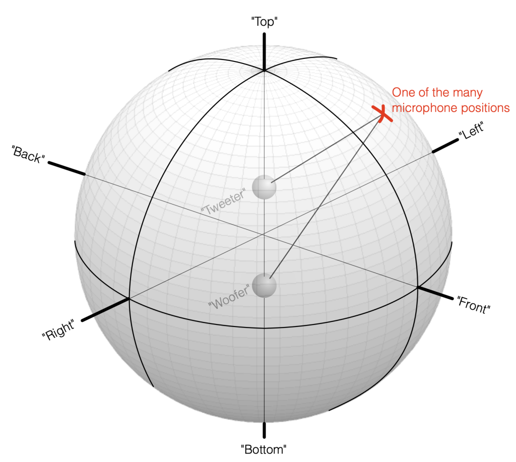
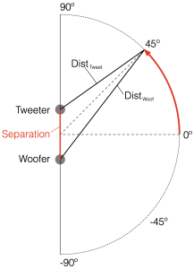
Take a look at Figure 7.1. I’ve now placed our two “perfect” omnidirectional point-source loudspeaker drivers in a three-dimensional space inside a giant sphere. I’ve called them a “tweeter” and a “woofer” again, just for the sake of clarity, but the truth is that I’m just treating them as full-range sources that are omnidirectional in all three dimensions.
We can then place our microphone at some location on the surface of that imaginary sphere, at some horizontal angle and some other vertical angle. You can consider the analysis I did in Part 6 to be a “slice” of this sphere, on the line that extends from the Bottom to the Top, running through the Front.
Sidebar
Put a real loudspeaker in your living room and listen to it from out in the kitchen while you make dinner. The loudspeaker radiates sound in all directions in all three dimensions, and that spherical ball of energy is more related to what you’ll hear bleeding into the kitchen than the simple on-axis response. No one is sitting in front of the loudspeaker, so there’s no one there to care about the on-axis response at all…
Let’s move microphone around the surface of that big sphere in Figure 7.1, making a measurement of the combined outputs of the tweeter and woofer (including the delay differences caused by the distance between the two loudspeaker drivers and the three-dimensional direction to the microphone) in each place. Since the two drivers are separated in space (among other things) they’ll result in a different measurement in each location. If we then combine all of those measurements to find the total magnitude response of the three-dimensional radiation, we’ll find the total Power Response of the system. This is the combined response of the loudspeaker’s output in all three dimensions, which is what we’re looking at in this article.
There are different ways to move around that sphere and then sum the numerous measurements that you get as a result. However, if you do the math correctly, it doesn’t really matter which way to do this.
I won’t say much more here; I’ll just show the plots. Each of the Figures below has three lines on it, showing three different separations between the two loudspeaker drivers. As in the previous postings, these are 0.125, 0.25, and 0.5 * the wavelength of the crossover frequency, which, in this case is 100 Hz.
This allows you to compare the tendency of the power response characteristic as the driver separation increases.
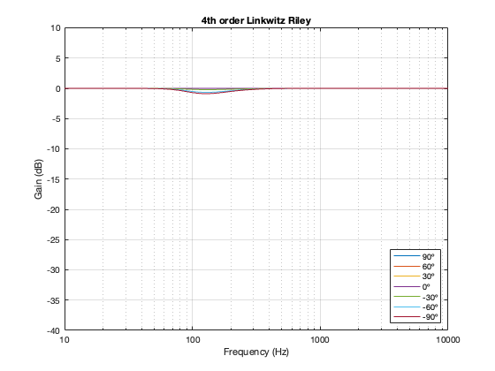
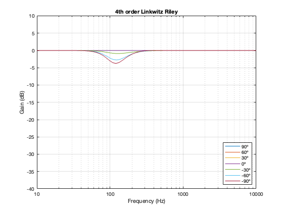
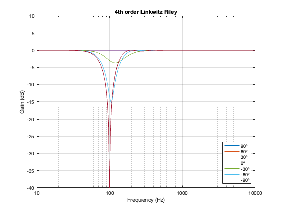
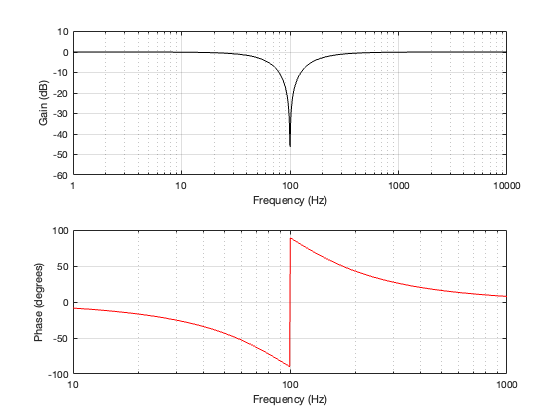
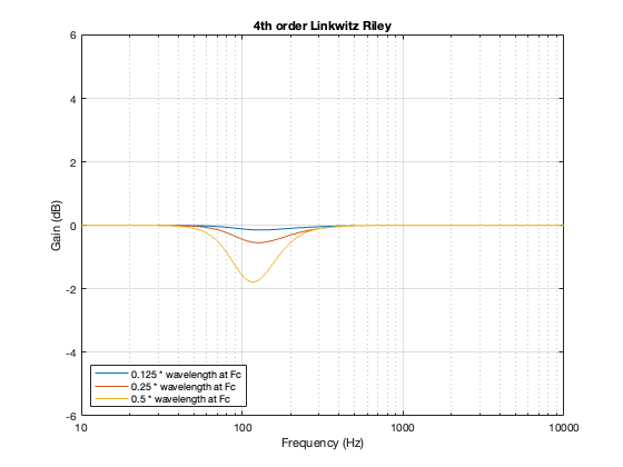
4th order Linkwitz Riley
Notice that the Power Response of the 4th-order Linkwitz Riley only drops in magnitude around the crossover frequency, and the depth and bandwidth of that dip is dependent on the distance between the drivers.
It’s also worth putting in the reminder here that if we moved the crossover to a different frequency, then the behaviour would look the same, just moved upwards or downwards on the x-axis. This is because I’m determining the distance between the two drivers using the wavelength of the crossover.
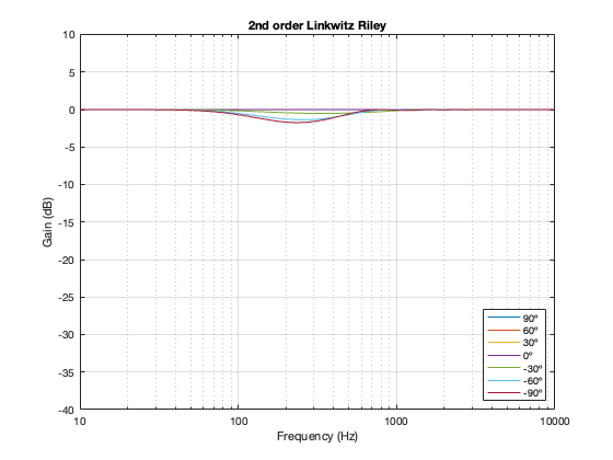
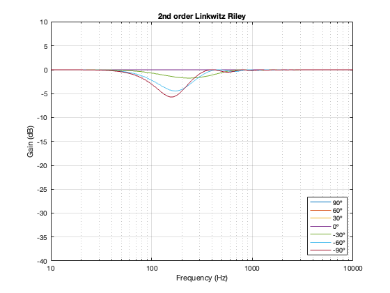
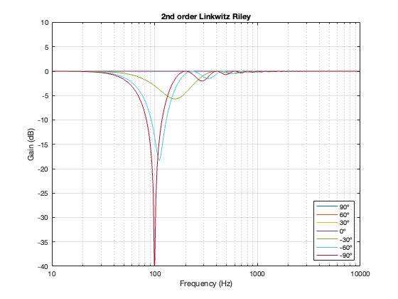
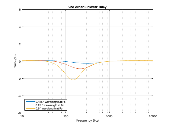
2nd order Linkwitz Riley
A 2nd-order Linkwitz Riley has a similar power response to the 4th order, although the effect is increased a little in frequency above the crossover, and it dips a little more for the same separation between the drivers.
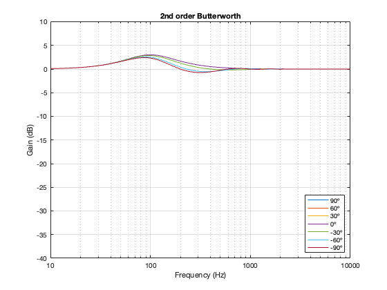
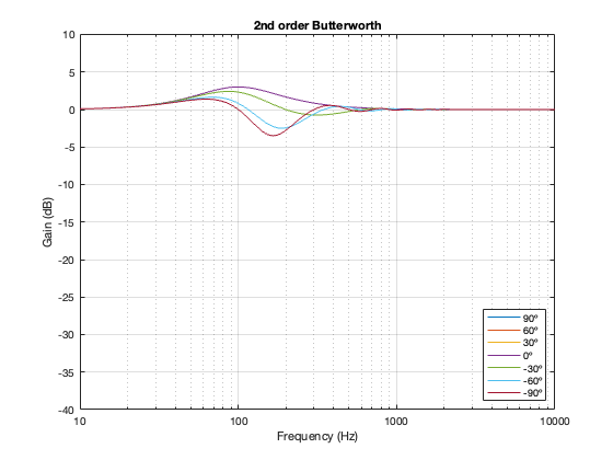
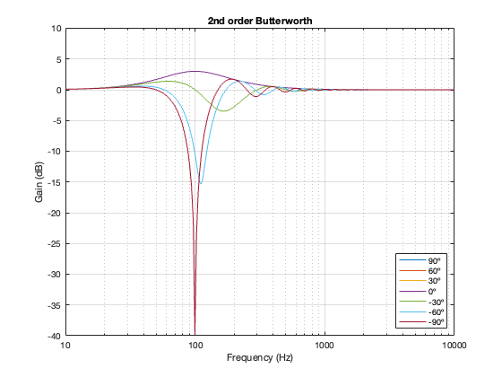
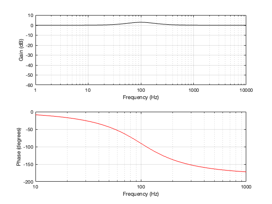
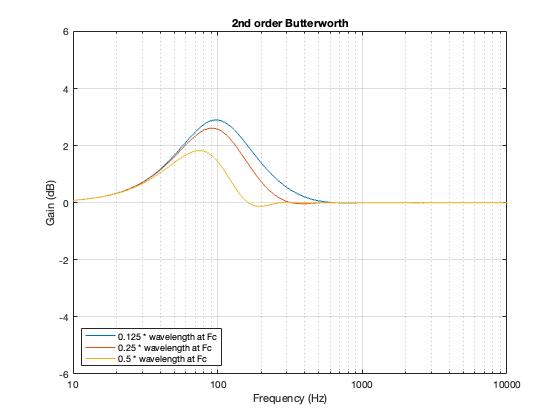
2nd order Butterworth
A 2nd-order Butterworth’s power response exhibits the opposite effect. It. produces a bump in around the crossover frequency instead of a dip. Also notice that the magnitude of the bump is more pronounced with the same distance between the loudspeaker drivers. Whereas a separation of 0.125*wavelength produced only a very slight dip in the power response for the two Linkwitz Riley crossovers, the same separation results in a more than 2 dB increase for the Butterworth design. Oddly, the bump gets smaller with larger separation – but this is a function of the relationship between the phase responses of the Butterworth filters and the delays of the two driver outputs at the various microphone positions around the sphere.
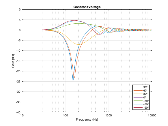
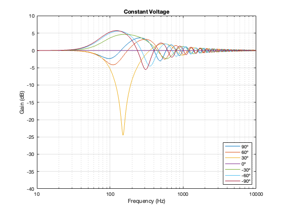
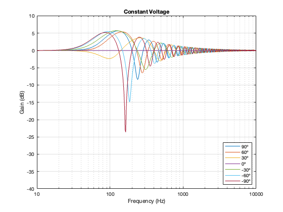
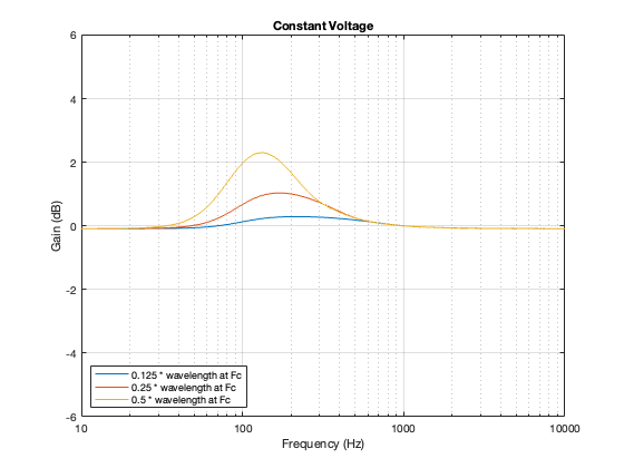
Constant Voltage
The constant voltage crossover is a little more intuitive in that the larger the separation between the drivers, the bigger the effect on the power response. In addition, it behaves similarly to the Butterworth design in that it produces a bump relative around (actually, just above) the crossover frequency.
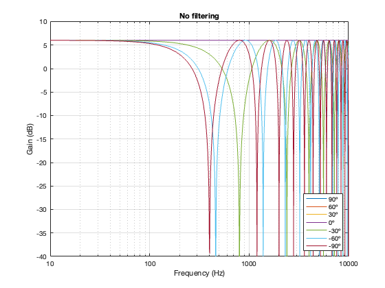
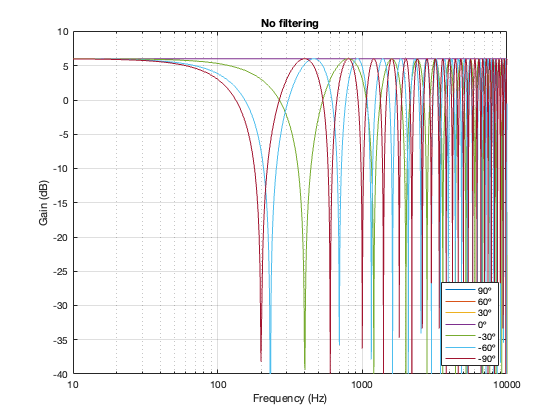
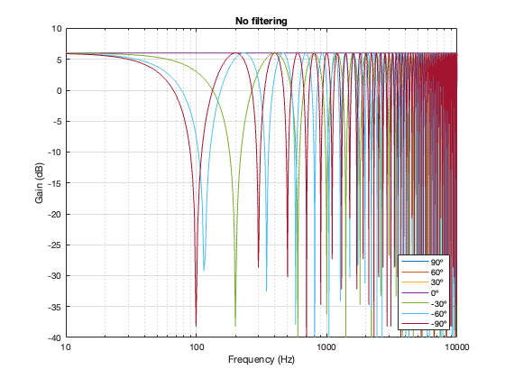
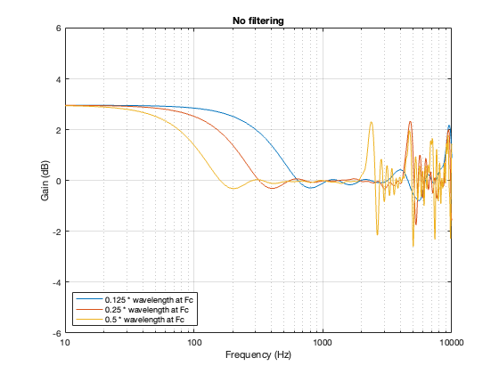
No Crossover
Again, just for curiosity’s sake, it’s interesting to look at the effect of having two drivers with the same separation as the models shown above, but without the filtering applied by a crossover. This is shown below in Figure 7.6. in the very low frequency band, you can see that the two drivers sum to give a 3 dB boost, which is equivalent to double the total power radiated by the system. The closer the two loudspeaker drivers are to each other, the higher the extension of this boost.
In addition, the strange effects in the high frequencies are essentially identical, but move up by one octave for each halving of distance between the drivers. You can also see that the interference effect is repeated each octave (notice the way that the orange and yellow lines overlap around 4 kHz, for example).
As I said in the sidebar above, if you do nothing but put in these crossover types, and your two loudspeakers are two little omnidirectional sources, then these plots will give you an idea of the difference in spectral balance that you’ll hear out in the kitchen when you play music. Of course, you would never do this. You would normally put in some extra filtering to fix things (whatever that means). In the next posting, we’ll look at what happens when you do that.