In the previous posting, I showed the frequency responses and impulse responses of the outputs of a crossover based on a linear phase filter strategy. One thing that can be seen in the impulse response plots in Figure 12.5 is that it never reaches a value of 0. It rings both backwards and forwards in time forever. However, this is not practical, since we don’t want to wait until the end of time to hear the output of our loudspeaker.
So, normally, we have to make a pragmatic choice about how long we’re willing to wait for the crossover filter’s to deliver an output. There are various ways to make this decision, but ultimately, we’re trying to balance the “error” in the responses of the crossover’s outputs with how long an input/output latency we’re willing to put up with. (We might also need to think about computational issues like how many calculations have to be done when you use a REALLY long filter, but I’m going to pretend that this is not an issue for this posting.)
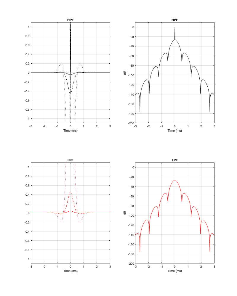
It’s difficult to see from a linear plot of the impulse responses of the two filters, but the peak is in the middle, at Time = 0 ms. Extending outwards, both backwards and forwards in time, the impulse responses oscillates back and forth across the 0-amplitude line. This oscillation is easier to see when it’s plotted in decibels, but then you can’t see whether the linear value is positive or negative. So, it helps to look at both to get an idea of what’s happening.
One thing that might not be immediately obvious is that, apart from the big spike at Time = 0 ms on the high-pass filter response, the outputs of the two filters are identical in amplitude, but opposite in polarity. In other words, they are symmetrical. This makes sense when you consider that, by adding them together, the total result is a single spike at Time = 0 and an amplitude of 0 at all other times. In other other words, the outputs of the two filters “cancel each other out” at all times except Time = 0.
This is a little weird if you think of it as the tweeter cancelling the woofer – but you consider that it’s doing it in time, at very low levels, then it might make more intuitive sense.
What happens if you don’t want to wait too long to get the output? In other words, if we shorten the impulse response around the central spike? This is a technique that is called “windowing” where you slice a window of time out of the middle of the impulse response and use only that.
There are a number of ways to do this. We could just say “everything up to 1 ms before the spike and everything after 1 ms after the spike, we just convert to silence”. This is the simplest way to do it, but it’s also the dumbest.
A smarter way is to look at the impulse response shown above, and fade into the spike and then fade back out again. Then you just decide on the shape of the fade and its length. It could be a straight line, or it could be something fancy.
I’ve written a lot about windowing in another posting a long time ago. If you want to learn about this topic, you could start there, or any book or website that talks about time-domain processing and analysis of audio signals. I won’t explain windowing in this posting. It’ll just get too long…
For all of the analyses below I did the following:
- Choose a crossover frequency
- Implement the crossover using linear phase filters
- Decide on a threshold in level (in dB below the spike at the input) to find out how long a window in time I’m going to use
- Apply a Hann window to the filters’ impulse responses with the length that I found above
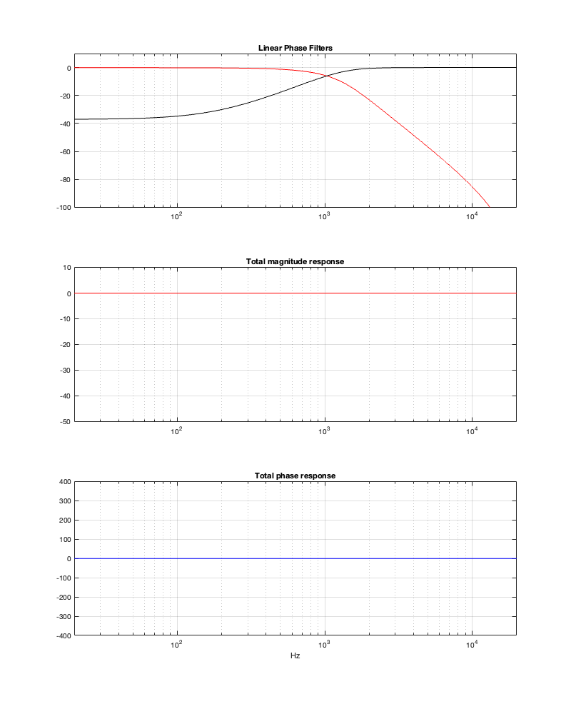
- Show the magnitude and phase responses of the individual outputs as well as the summed total
Another way to do this would be to just decide on the length of the windowing (and find out the threshold of the level, below which you’re cutting the signal) and see what happens. Either way, you get a deviation in the response, you’re just setting a different parameter.
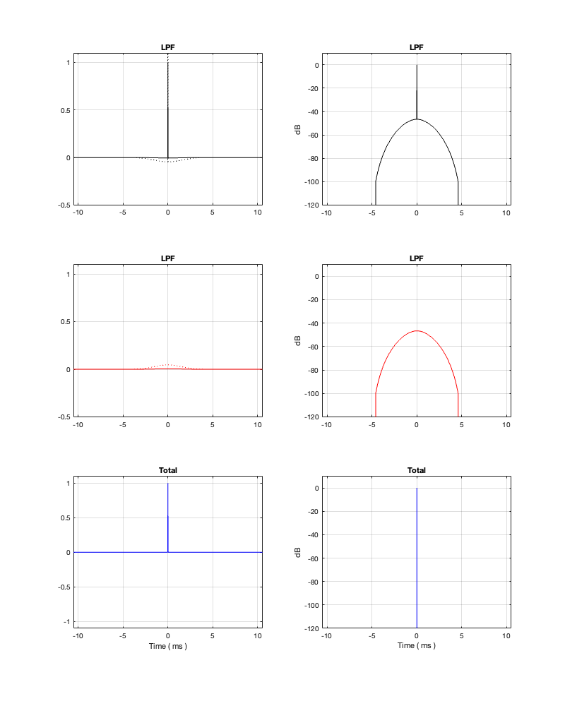
Fc = 1 kHz
Let’s start with a crossover frequency of 1 kHz. If I say that I want to extend the impulse response very far down in level, I’ll wind up getting a very accurate filter response (in other words, I’ll get what I expect), but it’ll have a long input/output latency (which is half of the total windowing time).

Minimum Latency = 5.44 ms
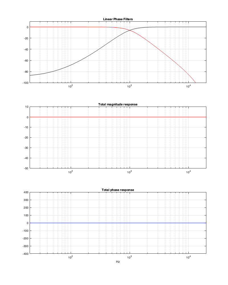
Hopefully, comparing the plot in Figure 13.1 and 13.2 helps to clarify the explanation above. Essentially, the plots in those two figures show the same thing. However, you can see in Figure 13.2 that I’ve cut off the impulse response once it drops below -250 dB.
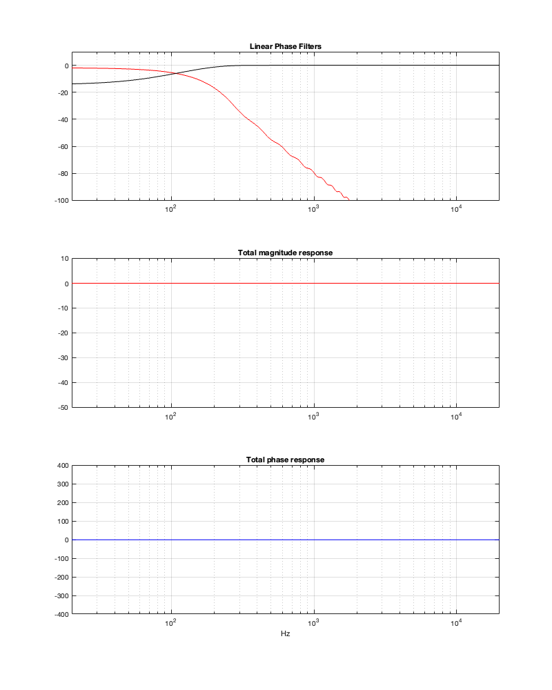
The effect of doing this windowing can be seen in Figure 13.3 where you can see that the roll-off for the tweeter doesn’t keep going down in level as you drop in frequency. This is because the lower the frequency you want to filter, the longer the filter’s impulse response has to be.
Notice, however, that, despite the fact that the two magnitude responses in the top of Figure 13.3 aren’t exactly what you’re expect, the responses of the summed total are what you’d expect. This will become a familiar theme as we continue.
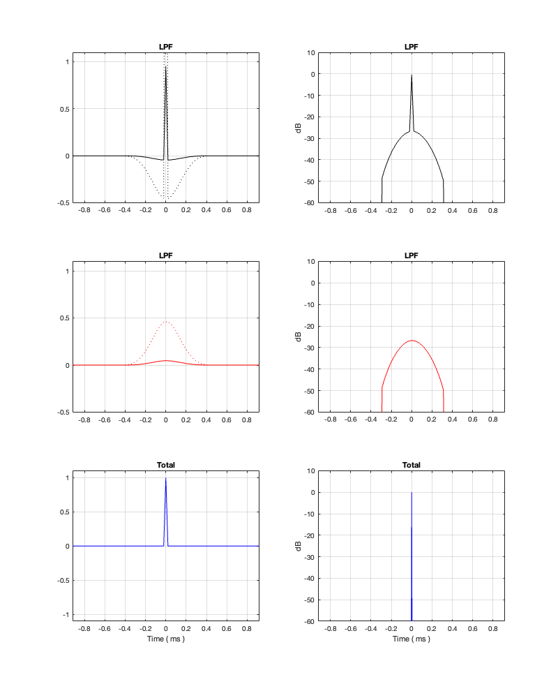
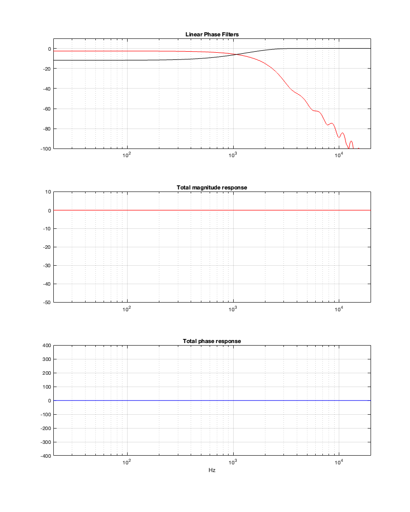
If we raise the threshold, we’ll shorten the impulse response, which means that we shorten the latency, and we deviate from the expected responses.
Minimum Latency = 1.23 ms
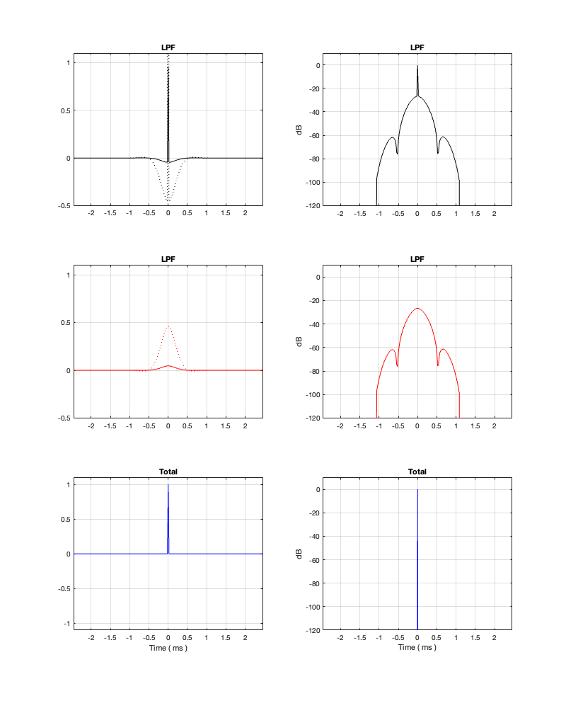
Notice in Figure 13.5 that, although the two crossover outputs have very different magnitude responses from 13.3, the total sum still works. Intuitively, this actually makes sense when you look at the impulse responses, since they still cancel each other – they’re just identical but opposite (except for the spike in the tweeter).
Of course, since the filter is now shorter in time, we get a lot more low-frequency output from the tweeter.
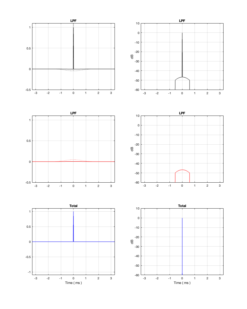
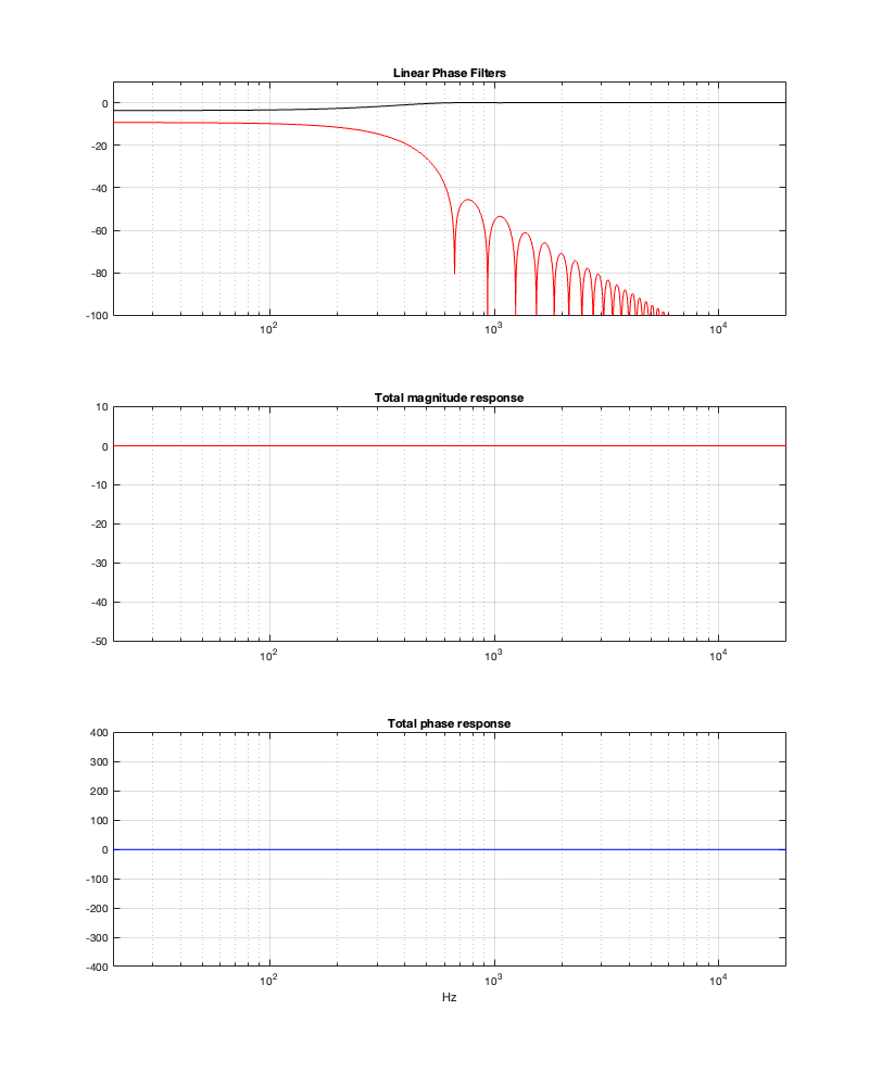
Minimum Latency = 0.46 ms
Notice in Figures 13.6 and 13.7 that, with a threshold of -50 dB, our latency can be under 0.5 ms. However, we will be expecting a lot of level out of the tweeter at low frequencies, which might be unhealthy for it if we turn up the volume.
Fc = 100 Hz
Now let’s repeat the process with a 100 Hz crossover to see what happens.
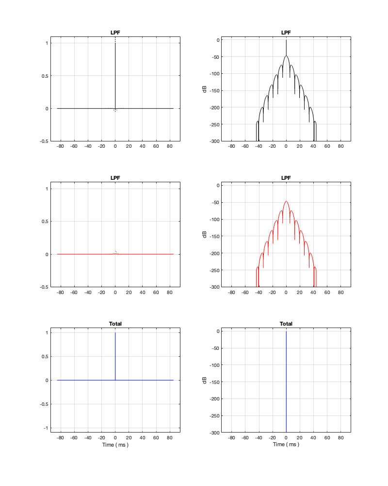
Minimum Latency = 47.58 ms
Notice that, in order to implement a threshold of -250 dB, we need at least about 47 ms of latency, which is probably outside acceptable limits for lip synch with video. It’s certainly far too long to be used in a loudspeaker for live sound, since you’ll hear and echo-echo all the time-time.
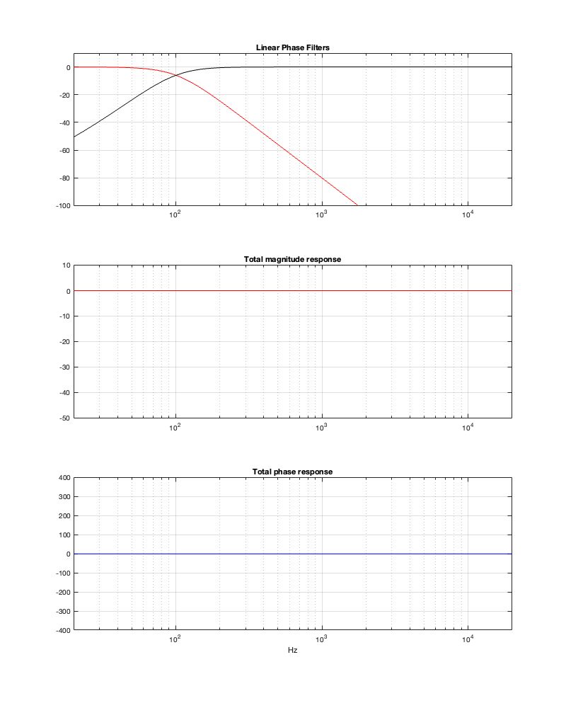
Minimum Latency = 5.27 ms
Notice that, by changing to a threshold of -100 dB, we’ve dropped our latency requirement significantly – down to just over 5 ms. However, don’t trust everything you see there. This crossover probably won’t behave nicely… If we change the threshold to -50 dB, you can see where we’re headed, and why I am highly suspicious of the -100 dB filters…
Minimum Latency = 1.65 ms
Obviously, that filter isn’t going to give you what you want – although it’ll give it to you quickly… (Editorial comment: It’s like current AI: it’s the fastest way to get the wrong answer…)
Wrapping up for now
Like I said above, regardless of how much I shorten these impulse responses, the responses of the summed outputs look good. This doesn’t necessarily mean that the crossover will work well, as should be evident by looking at the responses of the individual outputs.
In addition, it should be evident that, in order to implement a linear phase crossover that behaves well, you will incur a latency that may not be acceptable, depending on the crossover frequency and your requirements. Then again, if you don’t care about latency, you might start requiring a lot of computational power to implement it.
Like any aspect of crossover choice and design, there are multiple parameters to play with…
In the next posting, we’ll take a look at the implications of a linear phase crossover on the three-dimensional power response.