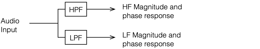
Up to now, we’ve either assumed that we don’t have any loudspeaker drivers in the chain (Parts 1 to 5 inclusive) or that our loudspeaker drivers are “perfect” point sources (Parts 6 to 8 inclusive). This means that, so far, our nice, perfect world has used a model that looks a little like Figure 9.1

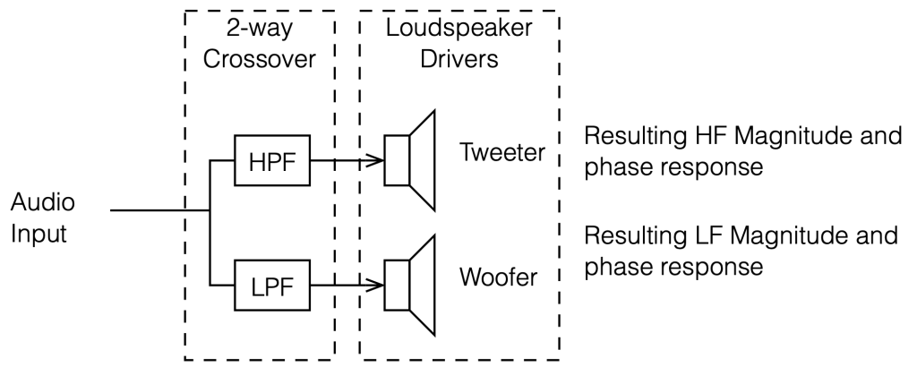
Now, we start getting a little closer to reality by adding some actual loudspeaker drivers to the outputs of the crossover. Going forward, I’m using the actual measurements of a real 1″ tweeter and a real 6″ woofer in a real sealed cabinet. So, now, instead of just looking at the magnitude and phase responses of the crossover’s outputs, we’re looking at the responses of the outputs of the drivers, as shown in Figure 9.2. Another way to think of this is that we have extra filters (the drivers’ responses, which are different in different directions) in addition to the filters in the crossover.

The problem with real loudspeakers is that they aren’t perfect, so let’s start by looking at their responses on-axis. These are shown in Figure 9.3

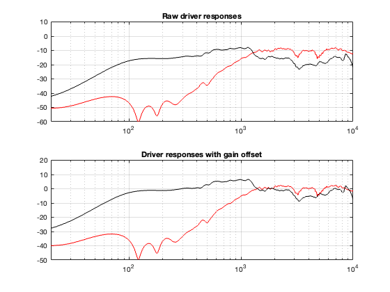
The top plot of Figure 9.3 shows the on-axis magnitude responses of the loudspeaker drivers in the cabinet without any filtering. The bottom plot shows the same responses, with gain offsets to match them at an arbitrary crossover frequency of 1800 Hz.

4th Order Linkwitz Reily

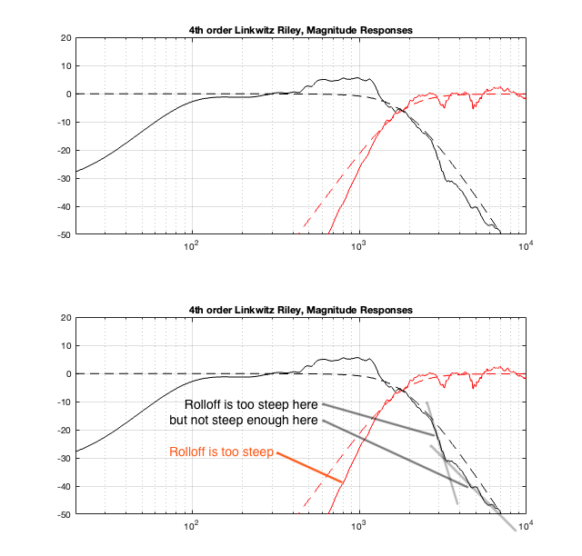
If I apply filtering using a 4th-order Linkwitz Reily crossover, and then send its outputs to a tweeter and a woofer, the resulting magnitude responses of the two drivers, when measured on-axis to the cabinet will look like the top plots in Figure 9.4, below.

I’ve duplicated the plot in the bottom half of the figure, and added some comments. Notice that the responses of the actual loudspeaker outputs, including the crossover filter, do NOT look like the theoretical responses of the crossover itself (shown as dotted lines). On-axis, the tweeter has a natural high-pass characteristic (seen in Figure 9.3) that, when combined with the high pass filter in the crossover, results in a slope that’s too steep.

The woofer’s rolloff is weird in that its contribution makes the low pass filter too steep at the start of the rolloff, and then not steep enough as you get a little higher in frequency. If you look back to Figure 9.3, this can be seen as the dip in the response that produces the “bowl” shape from roughly 1 kHz to 8 kHz.

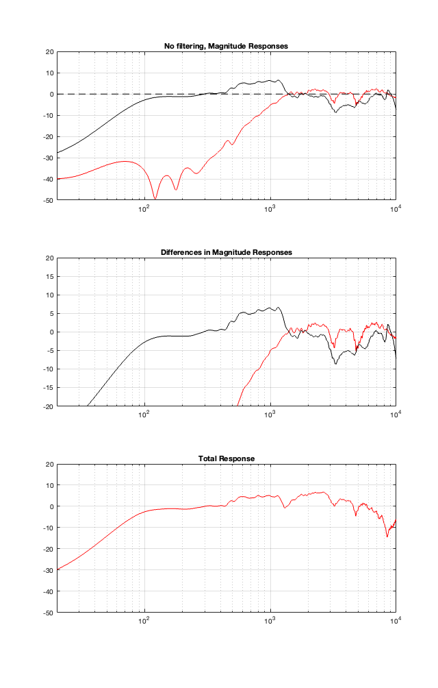
This means that, if we ignore the natural on-axis magnitude and phase responses of the loudspeaker drivers, and just slap a crossover in front of them, the resulting total response won’t be as pretty as we would expect. This is shown in the bottom plot in Figure 9.5.

The plots shown in the middle of Figure 9.5 are the difference between what we WANT the crossover to be (the dotted lines in the top plot) and the ACTUAL total resulting magnitude response at the outputs of the drivers (the solid lined in the top plot). In other words, these curves show the vertical distance between the solid and dotted lines in the top plot. If the drivers had perfectly flat magnitude responses, then these two lines would be flat, and they would sit on the 0 dB line.

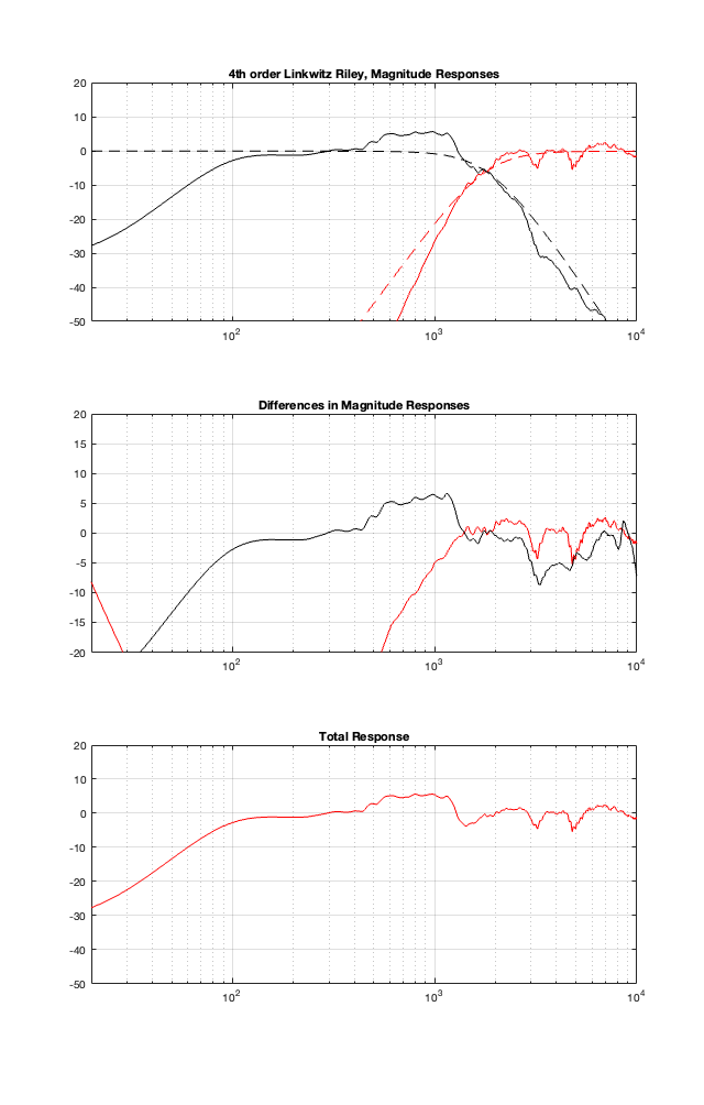
You might say that the Total Response in Figure 9.5 looks pretty good. I would disagree. An on-axis in-band magnitude response of about ±5 dB is pretty terrible if your goal is a flat on-axis response. If this is not your goal, then I have no opinion.

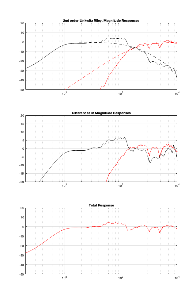
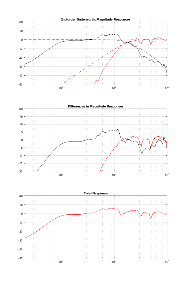
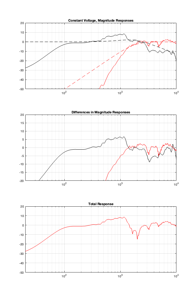
Now I’ll just throw in the same plots for the different crossover types, implementing the crossover with the assumption that the loudspeaker drivers are perfect, and then doing the analysis including the actual responses of the drivers.

2nd order Linkwitz Reily

2nd order Butterworth

Constant Voltage

No Crossover

Comparison

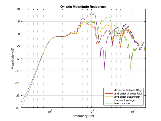
I’ll let you draw your own conclusions about the results of these plots. I will highlight one thing: remember that the theoretical combined magnitude responses of the 4th order Linkwitz Riley and the Constant Voltage crossovers are both flat. But compare their Total Responses in the plots above. Notice that they are very different from each other. This is, in part, because the phase responses of the two signal paths are modified by the driver’s behaviours, which means that they don’t add as nicely as we would like.

The moral of the story this time is: you can’t ignore the natural response of the drivers when you’re designing your crossover. This means that we will need to change our filters to ensure that the TOTAL response of the filter PLUS the driver results in the response that we want. The design of the crossover MUST include the responses of the drivers to ensure that it behaves as we wish.

But, so far, we have only considered this at one point in space, directly in front of the loudspeaker. In the next posting, we’ll come back to looking at the total power response. Things are about to get ugly…