Constant Voltage design
The four crossover types we’ve looked at so far all use the same basic concept: take the input signal and divide it into different frequency bands using some kind of filters that are implemented in parallel. You send the input to a high pass filter to create the high-frequency output, and you send the same input to a low-pass filter to create the low-frequency output.
In all of the examples we’ve seen so far, because they have been based on Butterworth sections, incur some kind of phase shift with frequency. We’ll talk about this more later. However, the fact that this phase shift exists bothers some people.
There are various ways to make a crossover that, when you sum its outputs, result in a total that is NOT phase shifted relative to the input signal. The general term for this kind of design is a “Constant Voltage” crossover (see this AES paper by Richard Small for a good discussion about constant voltage crossover design).
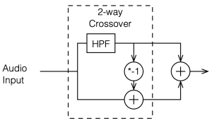
Let’s look at just one example of a constant voltage crossover to see how it might be different from the ones we’ve looked at so far. To create this particular example, I take the input signal and filter it using a 2nd-order Butterworth high pass. This is the high-frequency output of the crossover. To create the low-frequency output of the crossover, I subtract the high-frequency output from the input signal. This is shown in the block diagram below in Figure 5.1
As with the previous four crossovers, I’ve added the two outputs of the crossover back together to look at the total result.
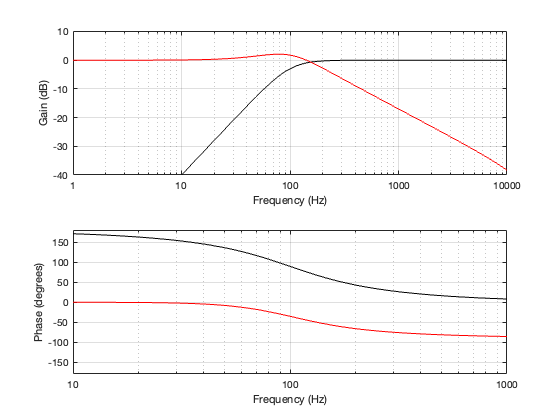
Figure 5.2 shows the magnitude and phase responses of the high- and low-frequency portions of the crossover. One thing that’s immediately noticeable there is that the two portions are not symmetrical as they have been in the previous crossover types. The slopes of the filters don’t match, the low-pass component has a bump that goes above 0 dB before it starts dropping, and their phase responses do not have a constant difference independent of frequency. They’re about 180º apart in the low end, and only about 90º in the high end.
However, because the low-frequency output was created by subtracting the high-frequency component from the input, when we add them back together, we just get back what we put in, as can be seen in Figure 5.3.
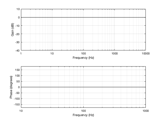
Essentially, this shows us that Output = Input, which is hopefully, not surprising.
If we then run our three sinusoidal signals through this crossover and look at the summed output, the results will look like Figures 5.4 to 5.6
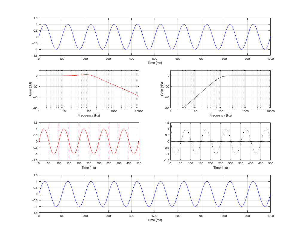
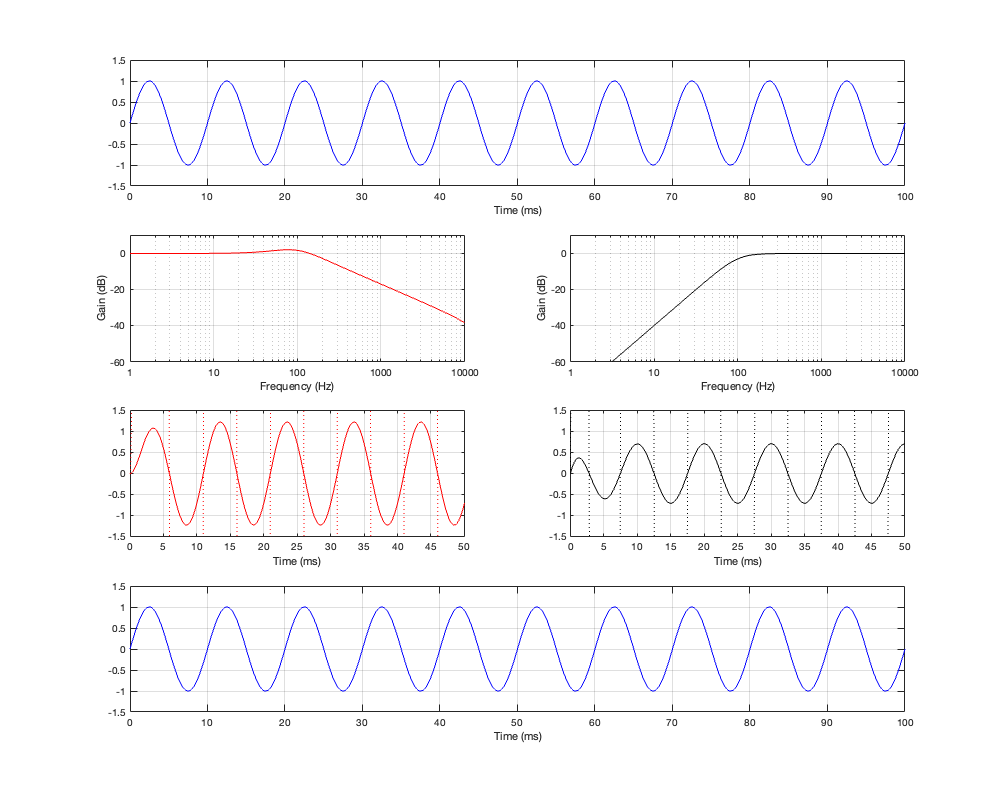
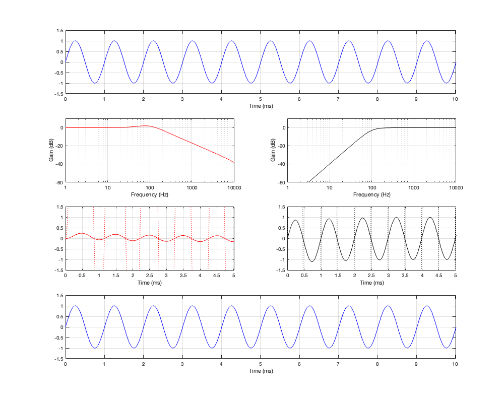
Notice in all three of those figures that the outputs and the inputs are identical, even though the individual behaviours of the two frequency-limited outputs might be temporarily weird (look at the start of the signals of the high-frequency output in Figures 5.4 and 5.6 for example…)
Now, don’t go jumping to conclusions… Just because the sum of the output is identical to the input of a constant voltage crossover does NOT make this the winner. We’re just getting started, and so far, we have only considered a very simple aspect of crossovers that, although necessary to understand them, is just the beginning of considering what they do in the real world.
Up to now, we have really only been thinking about crossovers in three dimensions: Frequency, Magnitude, and Phase. Starting in the next posting, we’ll add three more dimensions (X,Y, and Z of physical space) to see how, even a simple version of the real world makes things a lot more complicated.