One way to look at the behaviour of a signal when it’s sent through a crossover is to pretend that the loudspeaker isn’t part of the system. Once-upon-a-time, I probably would have phrased this differently and said something like “pretend that the loudspeaker is perfect”, but, now that I’m older, my opinions about the definition of “perfect” have changed.

So, we’ll take a signal, send it to a two-way crossover of some kind, and then just add the two signals back together. This shows us one view of the behaviour of the crossover, which is good enough to deal with the basics for now. In a later posting in this series, we’ll look at a more multi-dimensional and therefore realistic view of what’s happening.

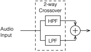
The block diagram above shows the signal flow that I used for all of the following plots in this posting.

Butterworth, 2nd-order (12 db/octave)

Although the block diagram above shows that we have a high-pass and a low-pass filter to separate the signal into two frequency bands, there are a lot of details missing about the specific characteristics of those filters. There are many ways to make a high-pass filter, for example…

One common crossover type uses 2nd-order Butterworth filters, both with the same cutoff frequency. One way to implement these are to use biquads to make low-pass and high-pass filters with Q = 1/sqrt(2).

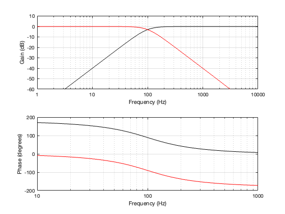
Before we look at the output of the entire crossover after the two signals have been summed, let’s talk about the red and the black curves in the plots above.

The magnitude responses should not come as a surprise. The fact that I’m using 2nd-order filters means that the slope of the attenuation will be 12 dB per octave (or 40 dB per decade) once you get far enough away from the cutoff frequency. The fact that they also have a Q of 1/sqrt(2) (approximately 0.707) means that they will attenuate the signal by 3 dB at the cutoff frequency, and that there is no “bump” in the slope of the magnitude response.

However, the phase responses might be a little confusing. Let’s take those separately:

For the low-pass filter (the black line), you can see that in the high-frequency band, where the magnitude response is a flat line at 0 dB (which means that the level of the output level is equal to the level of the input), the phase shift is 0º.

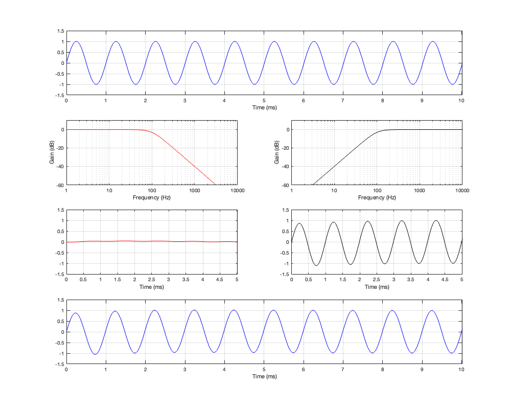
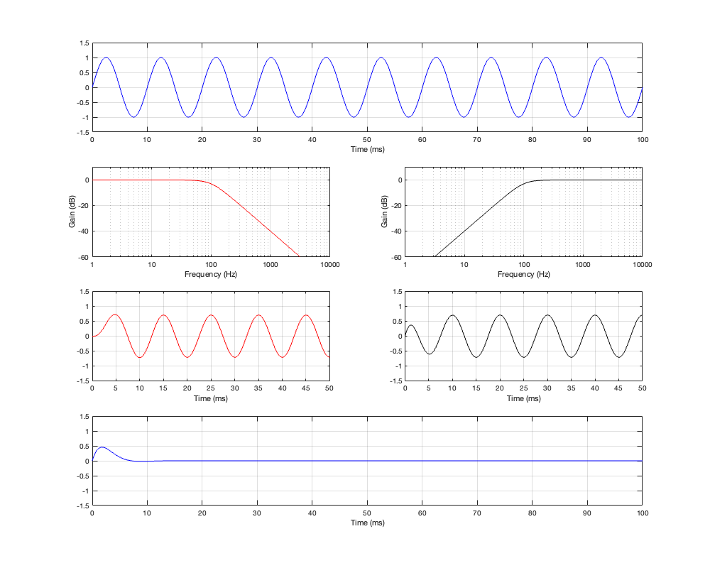
Another way to look at this is to put a sine wave into the system and see what comes out, as shown in Figure 2.3 below. The top plot shows the input to the two filters. Since this sine wave has a period of 1 ms, then it’s a 1000 Hz tone.

The second row of plots shows the magnitude responses of the low-pass filter (in red, on the left) and the high-pass filter (in black, on the right). Notice the levels of these two curves at a frequency of 1000 Hz.

The third row of plots shows the actual outputs of the two filters. For now, we’ll only look at the output of the high-pass filter on the right. There are three things to notice about this plot:

• After about 1 ms, the amplitude of this sine tone is the same as the one in the top plot.
• The phase of this sine tone is the same as the one in the top plot. In other words (for example), they both pass the 0 line, heading positive at Time = 1 ms.
• The start of the sine wave is a little weird. Notice that the positive peak is lower than expected and first negative trough is BELOW the maximum-negative amplitude. (it’s below a value of -1).
  We’ll ignore this for now, and come back to it later.

The fourth row shows the output of the two filters when they have been added together. Notice here that the output is almost identical to the input because it’s essentially just the contribution of the high-pass filter. The low-pass filter has so little output that it’s practically irrelevant.

Let’s now look a what happens if we put in a low-frequency sine wave instead. This is shown in Figure 2.4.

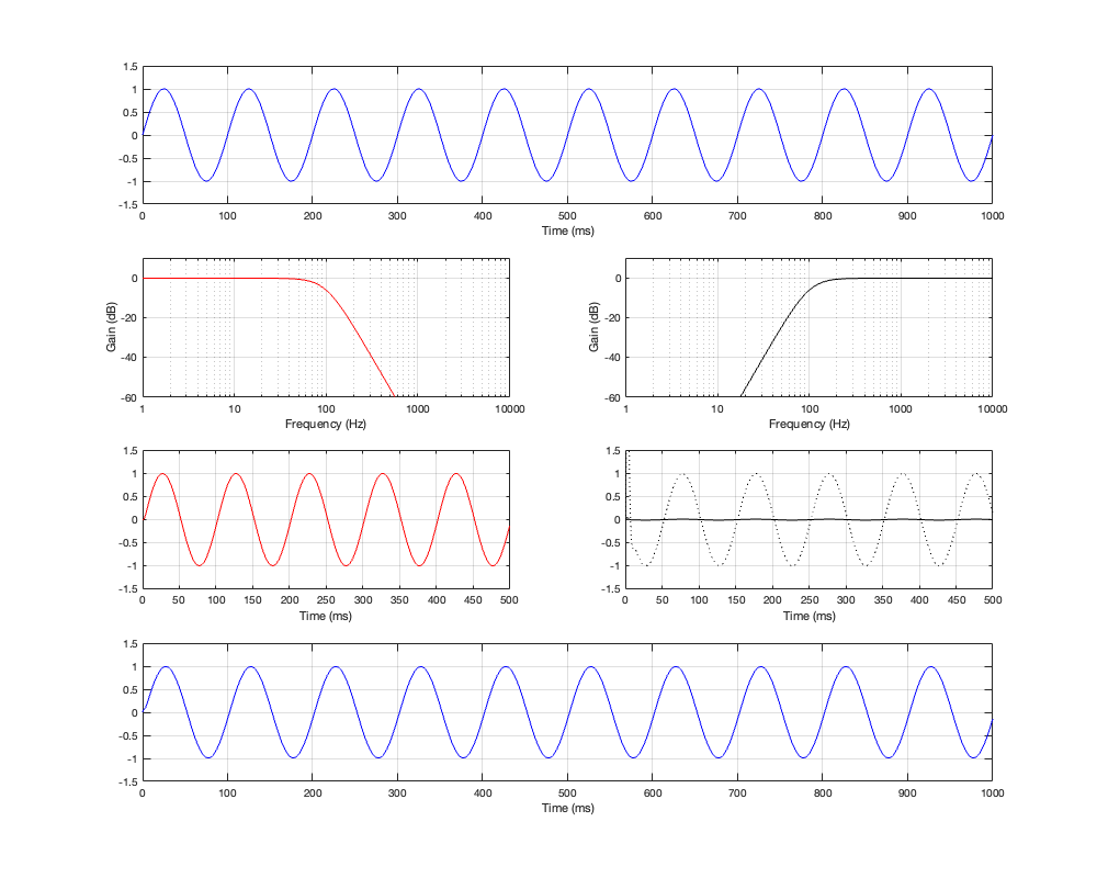
Notice now that the time scale is 100 times longer. The sine wave now has a period of 100 ms, so it’s a 10 Hz sine wave.

We’ll focus on the third row of plots again, still looking only at the output of the high-pass filter on the right. There are three things to notice about this plot:

• After about 100 ms, the amplitude of this sine tone (the solid black line) is MUCH lower than the amplitude of the input. The dotted line is a “magnified” version of the same signal so that we can see it for the phase comparison.
• The phase of this sine tone is the shifted by 180º relative to the top plot. In other words (for example), at Time = 200 ms they both pass the 0 line, but this signal is going negative when the input is going positive.
• The start of the sine wave is a also weird, but differently so; with that spike at the beginning and the weird wiggle in the curve before it settles down.
  We’ll ignore this for now, and come back to it later.

If you go back and look at the low-pass filter’s output, then you’ll see basically the same behaviour, but for the opposite frequency.

And, again, the output is almost identical to the input because it’s essentially just the contribution of the low-pass filter. The high-pass filter has so little output that it’s practically irrelevant.

Now let’s look at what happens when the frequency of the input signal is on the cutoff frequency of the two filters – in other words, the crossover frequency.

Now the sine wave has a period of 10 ms, so its frequency is 100 Hz.

Take a look at the third row of plots at Time = 10 ms.

The first thing to do is to compare the outputs of the two filters. The output of the low-pass filter on the left is negative, whereas the output of the high-pass filter on the right is positive. The outputs of the two filters are 180º out of phase with each other. This can also be seen in the plot back in Figure 2.2, where it’s shown that the difference between the red and the black phase response plots is 180º at all frequencies.

This is also why., once everything settles down, the sum of the two filters (the blue line on the bottom) is silence. The two signals have equal amplitude, and are 180º out of phase, so they cancel each other out.

Now compare those signal plots in the third row in Figure 2.5 to the input signal shown in the top plot. If you look at Time = 10 ms again (for example), you can see that the output of the low-pass filter is 90º behind the input. However, the output of the high-pass filter is early 90º ahead of the input.

The fact that the phase of the output of the high-pass filter is ahead of its own input confuses many people, however, don’t panic. This does not mean that the output is ahead of the input in TIME. The high-pass filter cannot see into the future. The only reason its output can have a phase that precedes the phase of its input is if the sine wave has been playing for a long time (and, in this case a “long” time can be measured in milliseconds…).

This confusion is the result of two things:

• People are typically taught the concept of phase as it relates to time. However, if you’re talking about a sine wave, then you are implying infinite time. in order for a signal to be a REAL sine wave, it must have always been playing and it must never stop. If it started or stopped, then there are other frequencies present, and so it’s not a theoretically-perfect sine wave.
• We use the words “ahead” and “behind” or “earlier” and “later” to describe the phase relationships, and these words typically imply a time relationship.

Maybe a rough analogy that can help is to walk next to a friend, at the same speed, but do not synchronise your steps. You will both arrive at the same place at the same time, but at two different moments in the cycles of your footsteps.

Of course, if you make a crossover like this, it won’t work very well, since you get that cancellation at the crossover frequency when the two filters outputs are added together. If we plot the summed response’s magnitude and phase characteristics, they look like the plots shown in Figure 2.6.

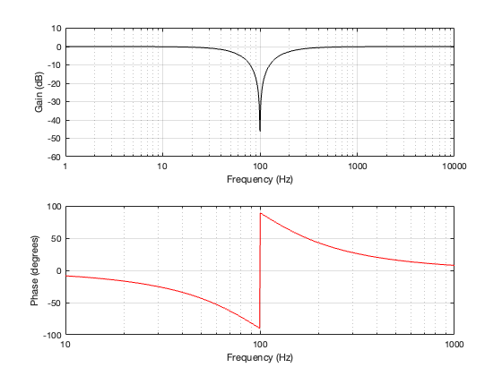
As you can see there, there is complete cancellation at the crossover frequency, and the phase response flips across that notch.

So, the solution with a 2nd-order Butterworth crossover is to assume that people won’t notice if you invert the polarity of the high-pass filter’s output. This is a good assumption that I will not argue with at all.

This polarity inversion “undoes” the 180º phase difference of the two filters seen in Figure 2.2, and the summed result is shown below in Figure 2.7 and 2.8.

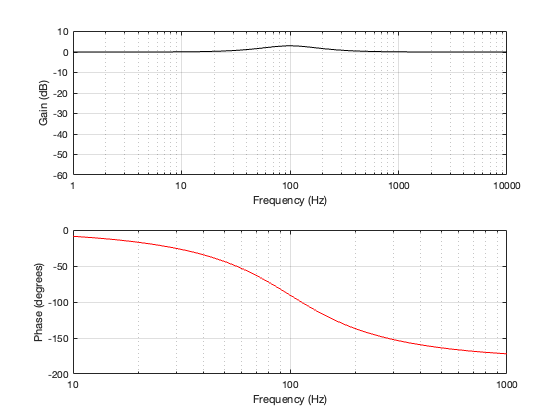
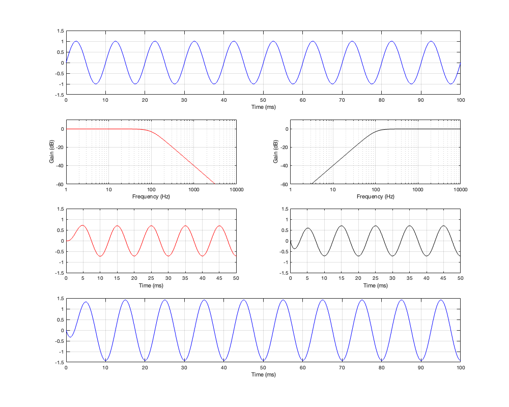
Now the outputs of the two filters appear to be in phase with each other. They are still 90º out of phase with the input, which means that their summed outputs are also 90º out of phase with the input. This can be seen in the bottom plots of Figure 2.7 and 2.8.

You’ll also notice that there is a 3 dB bump at the crossover frequency. This is because, at their cutoff frequencies, both filters attenuate by 3 dB (a linear gain of 0.707). When those two signals of equal amplitude and matching phase are added together, you get a magnitude that is 6 dB higher (or a linear gain of 1.41). We’ll talk about this later when we start looking at the real world.

Finally, take a look at the bottom plot in Figure 2.7. You can see there that the summed outputs of the two filters result in a phase shift that increases with frequency. In fact, when we look at a 2nd-order Butterworth crossover like this, without all the real-world implications of loudspeaker drivers that have their own characteristics and are separated in space, it can be seen that it acts as a 2nd-order minimum-phase allpass filter. This isn’t necessarily a bad thing, so don’t jump to conclusions this early…

We are STILL not going to talk about that weirdness at the beginning of the signal after it’s been filtered. That will come later.