#55 in a series of articles about the technology behind Bang & Olufsen loudspeakers

 

In a previous posting, I talked about the relationship between its “Bl” or “force factor” curve and the stiffness characteristics of its suspension and the fact that this relationship has an effect on the distortion characteristics of the driver. What was missing in that article was the details in the punchline – the “so what?” That’s what this posting is about – the effect of a particular kind of distortion in a system, and its resulting output.

 

WARNING: There is an intentional, fundamental error in many of the plots in this article. If you want to know about this, please jump to the “appendix” at the end. If you aren’t interested in the pedantic details, but are only curious about an intuitive understanding of the topic, then don’t worry about this, and read on. As an exciting third option, you could just read the article, and then read the appendix to find out how I’ve been protecting you from the truth…

 

Examples of Non-linear Distortion

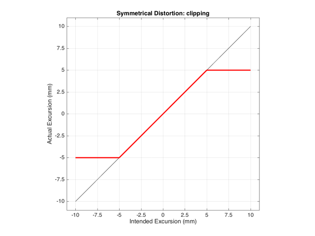
Let’s start by looking at something called a “transfer function” – this is a plot of the difference between what you want and what you get.

For example, if we look at the excursion of a loudspeaker driver: we have some intended excursion (for example, we want to push the woofer out by 5 mm) and we have some actual excursion (hopefully, it’s also 5 mm…)

If we have a system that behaves exactly as we want it to within some limit, and then at that limit it can’t move farther, we have a system that clips the signal. For example, let’s say that we have a loudspeaker driver that can move perfectly (in other words, it goes exactly where we want it to) until it hits 5 mm from the rest position (either inwards or outwards). In this case, its transfer function would look like Figure 1.

 

 

This means that if we try to move the driver with a sinusoidal wave that should peak at 10 mm and -10 mm, the tops and bottoms of the wave will be “chopped off” at ±5 mm. This is shown in Figure 2, below.

 

 

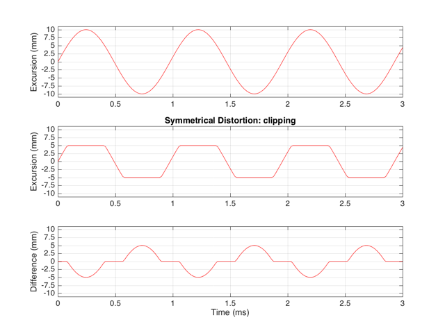
Let’s think carefully about the bottom plot in Figure 2. This is the difference between the actual excursion of the driver and the desired excursion (I calculated it by actually subtracting the top plot from the middle plot) – in other words, it’s the error in the signal. Another way to think of this is that the signal produced by the driver is what you want (the top plot) PLUS the error (the bottom plot). (Looking at the plots, if middle-top = bottom, then top+bottom = middle)

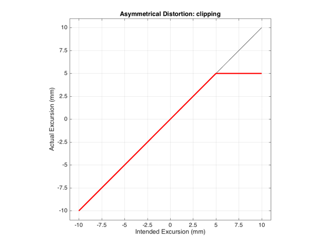
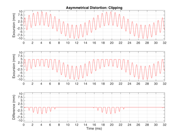
These plots show a rather simple case where the clipping of the signal is symmetrical. That is to say that the error on the positive part of the waveform is identical to that on the negative part of the waveform. As we saw in this posting, however, perfectly symmetrical distortion is not guaranteed… So, what happens if you have asymmetrical distortion? Let’s say, for example, that you have a system that behaves perfectly, except that it cannot move more than 5 mm outwards (moving inwards is not limited). The transfer function for this driver would look like Figure 3.

 

 

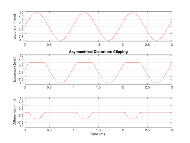
How would a sinusoidal waveform look if it were passed through that driver? This is shown in Figure 4, below.

 

As we also saw before, it is unlikely that the abrupt clipping of a signal is how a real driver will behave. This is because, usually, a driver has an increasing stiffness and a decreasing force to push against it, as the excursion increases. So, instead of the driver behaving perfectly to some limit, and then clipping, it is more likely that the error is gradually increasing with excursion. An example of this is shown below in Figure 5. Note that this plot is just a tanh (a hyperbolic tangent) function for illustrative purposes – it is not a measurement of a real loudspeaker driver’s behaviour.

 

 

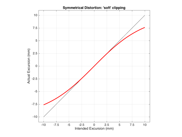
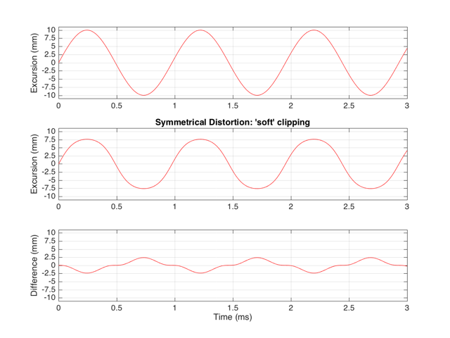
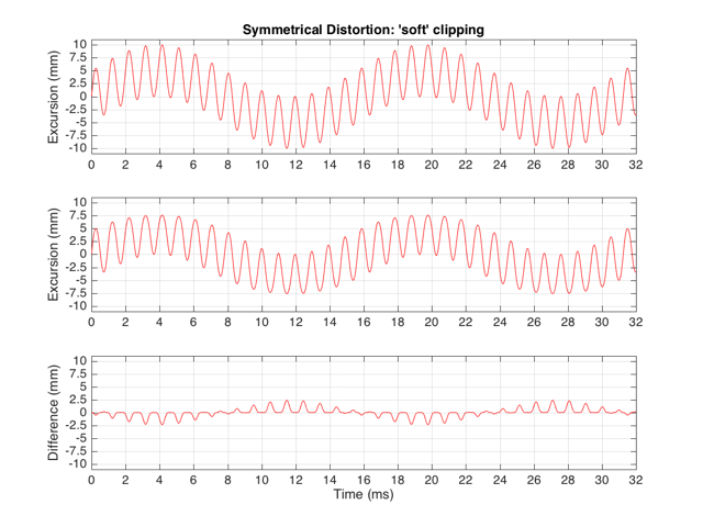
If we were to pass a sinusoidal waveform through this system, the result would be as is shown in Figure 6.

 

 

 

Harmonic Distortion

The reason engineers love sinusoidal waveforms is that they only contain one frequency each. A 1000 Hz sine tone only has energy at 1000 Hz and no where else. This means that if you have a box that does something to audio, and you put a 1000 Hz sine tone into it, and a signal with frequencies other than 1000 Hz comes out, then the box is distorting your sine wave in some way.

This was a very general statement and should be taken with a grain of salt. A gain applied perfectly to a signal is also a distortion (since the output is different from the input), but will not necessarily add new frequency components (and therefore it is linear distortion, not non-linear distortion). A box that adds noise to the signal is, generally speaking, distorting the input – but the output’s extra components are unrelated to the input – which would classify the problem as noise instead of distortion.) To be more accurate, I would have said that “if you have a box that does something to audio, and you put a 1000 Hz sine tone into it, and a signal with frequencies other than 1000 Hz comes out, then the box is applying a non-linear distortion to your sine wave in some way.”

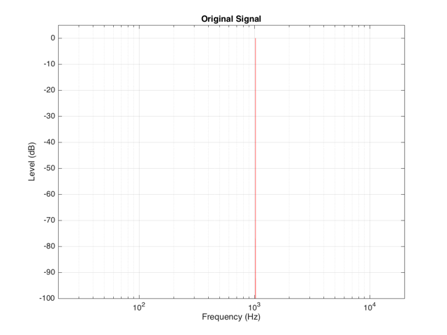
Back to the engineers… If you take a sinusoidal waveform and plot its frequency content, you’ll see something like Figure 7. This shows the frequency content of a signal consisting of a 1024 Hz sine wave.

 

 

If we clip this signal symmetrically, using the transfer function shown in Figure 1, resulting in the signal shown in the middle plot in Figure 2, and them measure the frequency content of the result, it will look like Figure 8.

 

 

There are at least two interesting things to note about the frequency content shown in Figure 8.

The first is that the level of the signal at the fundamental frequency “f” (1024 Hz, in this case) is lower than the input. This might be obvious, since the output cannot “go as loud” as the input of the system – so some level is lost. (Since we’re clipping at -6 dB, the fundamental has dropped by 6 dB.)

The second thing to notice is that the new frequencies that have appeared are at odd multiples of the frequency of the original signal. So, we have content at 3072 Hz (3*1024), 5120 Hz (5*1024), 7168 Hz (7*1024) and so on. This is a characteristic of a symmetrically distorted signal (meaning not only that we have distorted the top and the bottom of the signal in the same way, but also that the signal itself was symmetrical to begin with). In other words, whenever you see a distortion product that only produces odd-order harmonics of the fundamental, you have a system that is distorting a symmetrical signal symmetrically.

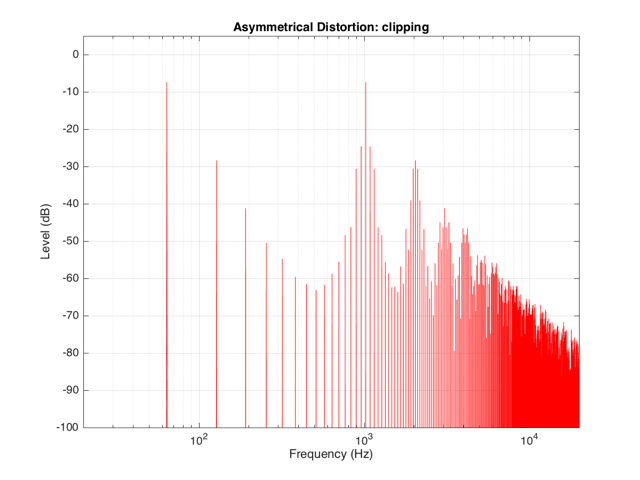
If we were to look at the frequency content of the asymmetrically-distorted signal (shown in Figures 3 and 4), the result would be as is shown in Figure 9.

 

 

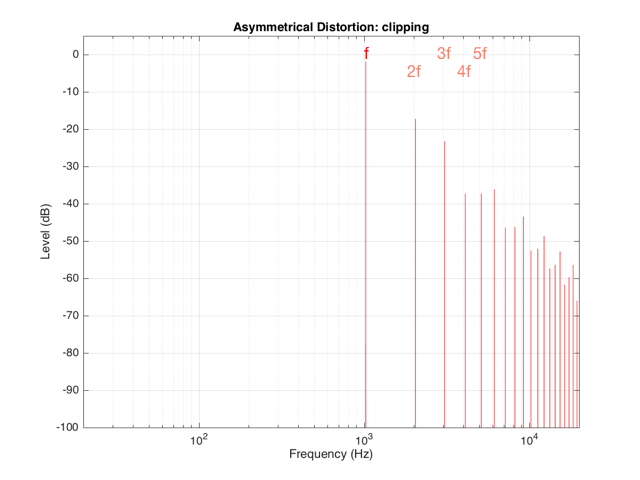
In Figure 9, you can see at least two interesting things:

The first is that the level of the fundamental frequency of “f” (1024 Hz) is higher than it was in Figure 8. This is because we’re letting more of the energy of the original waveform through the distortion (because the negative portion is untouched).

The second thing that you can see in Figure 9 is that both the odd-order and the even-order harmonics are showing up. So, we get energy at 2048 Hz (2*1024), 3072 Hz (3*1024), 4096 Hz (4*1024), 5120 Hz (5*1024), and so on. The presence of the even-order harmonics tells us that either the input signal was asymmetrical (which it wasn’t) or that the distortion applied to it was asymmetrical (which is was) or both.

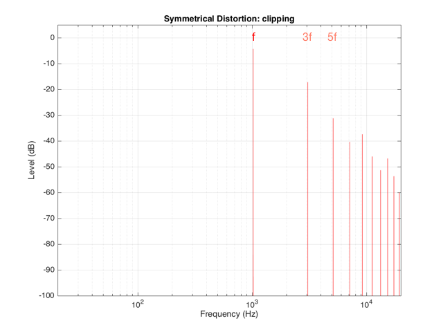
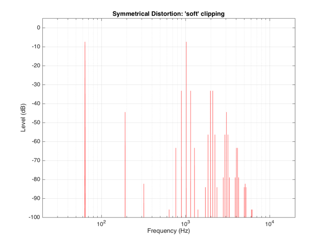
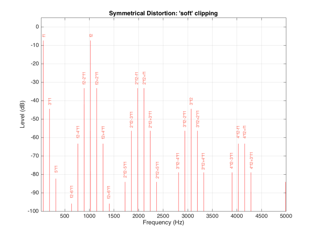
If the distortion we apply to the signal was less abrupt – using the “soft-clipping” function shown in Figure 5 and 6, the result would be different, as is shown in Figure 10.

 

 

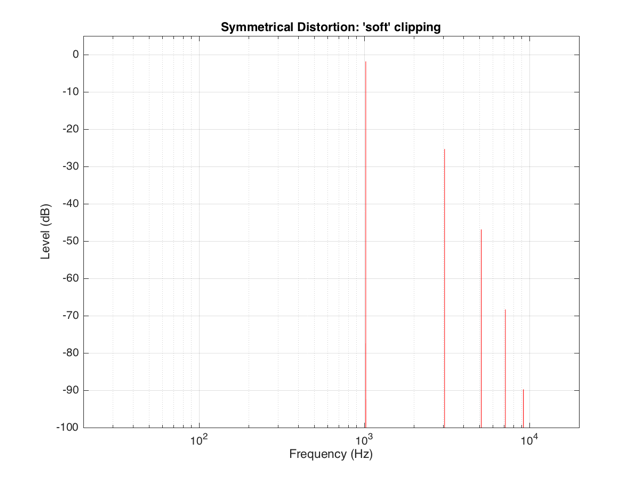
Again, in Figure 10, you can see that only the odd-order harmonics appear as the distortion products, since the distortion we’re applying to the symmetrical signal is symmetrical.

 

Intermodulation Distortion

So far, we’ve only been looking at the simple case of an input signal with a single frequency. Typically, however, research has shown that most persons listen to more than one frequency simultaneously (acoustical engineers and Stockhausen enthusiasts excepted…). So, let’s look at what happens when we have more than one frequency – say, two frequencies – in our input signal.

For example, let’s say that we have an input signal, the frequency content of which is shown in Figure 11, consisting of sinusoidal tones at 64 Hz and 1024 Hz. Both sine tones, individually, have a peak level of one-half of the maximum peak of the system. Therefore, they are shown in Figure 11 as having a level of approximately -6 dB each.

 

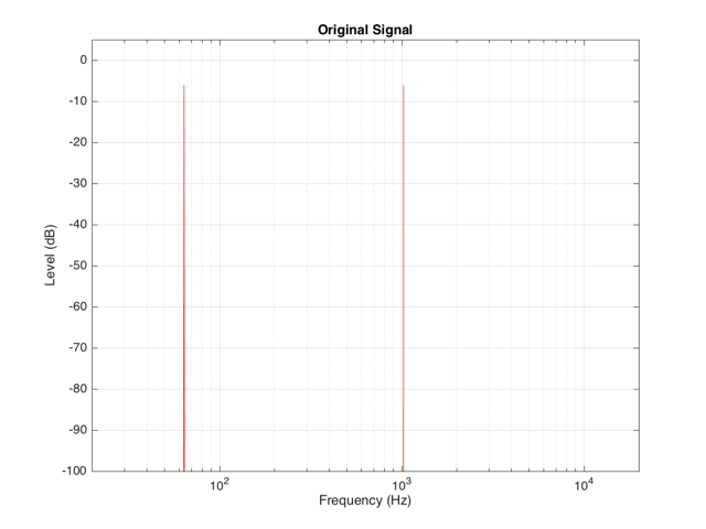
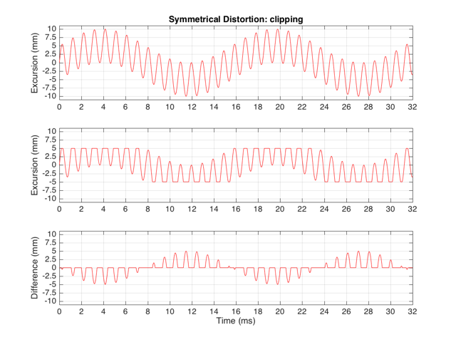
The sum of these two sinusoids will look like the top plot in Figure 12. As you can see there, the signal with the higher frequency is “riding on top of” the signal with the lower frequency. Each frequency, on its own, is pushing and pulling the excursion by ±5 mm. The total result therefore can move from -10 mm to +10 mm, but its instantaneous value is dependent on the overlap of the two signals at any one moment.

If we apply the symmetrical clipping shown in Figure 1 to this signal, the result is as is shown in the middle plot of Figure 12 (with the error shown in the bottom plot). This results in an interesting effect since, although the distortion we’re applying should be symmetrical, the result at any given moment is asymmetrical. This is because the signal itself is asymmetrical with respect to the clipping – the high frequency component alternates between getting clipped on the top and the bottom, depending on where the low frequency component has put it…

 

 

We can look at the frequency content of the resulting clipped signal. This is shown in Figure 13.

 

 

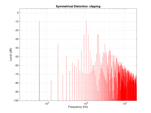
It’s obvious from the plot in Figure 13 that we have a mess. However, although the mess is rather systematic, it’s difficult to see in that plot. If we plot the same information on a different scale, things get easier to understand. Take a look at Figure 14.

 

 

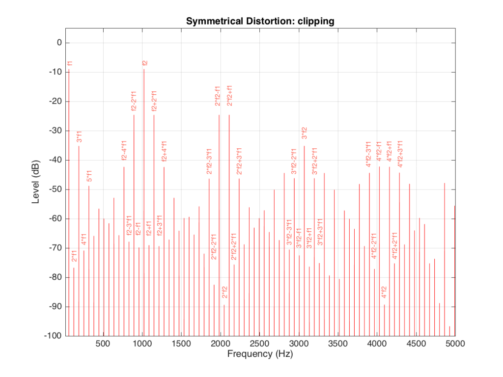
Figure 14 and Figure 13 show exactly the same information with only two differences. The first is that Figure 14 only shows frequencies up to 5 kHz instead of 20 kHz. The second is that the scale of the x-axis of Figure 13 is logarithmic whereas the scale of Figure 14 is linear. This is only a chance in spacing, but it makes things easier to understand.

As you can see in Figure 14, the extra frequencies added to the original signal by the clipping are regularly spaced. This is because the distortion that we have generated (called an intermodulation distortion, since it results from two two signals modulating each other), in the frequency domain, follows a pretty simple mathematical pattern.

Our original two frequencies of 64 Hz (called “f1” on the plot) and 1024 Hz  (“f2”) are still present.

In addition, the sum and difference of these two frequencies are also present (f2+f1 = 1088 Hz and f2-f1 = 1018 Hz).

The sum and difference of the harmonic distortion products of the frequencies are also present. For example, 2*f2+f1 = 2*1024+64=2112 Hz, 3*fs-2*f1 = 3*1024-2*64 = 2944 Hz…  There are many, many more of these. Take one frequency, multiply it by an integer and then add (or subtract) that from the other frequency multiplied by an integer – whatever the result, that frequency will be there. Don’t worry if your result is negative – that’s also in there (although we’re not going to talk about negative frequencies today – but trust me, they exist…)

 

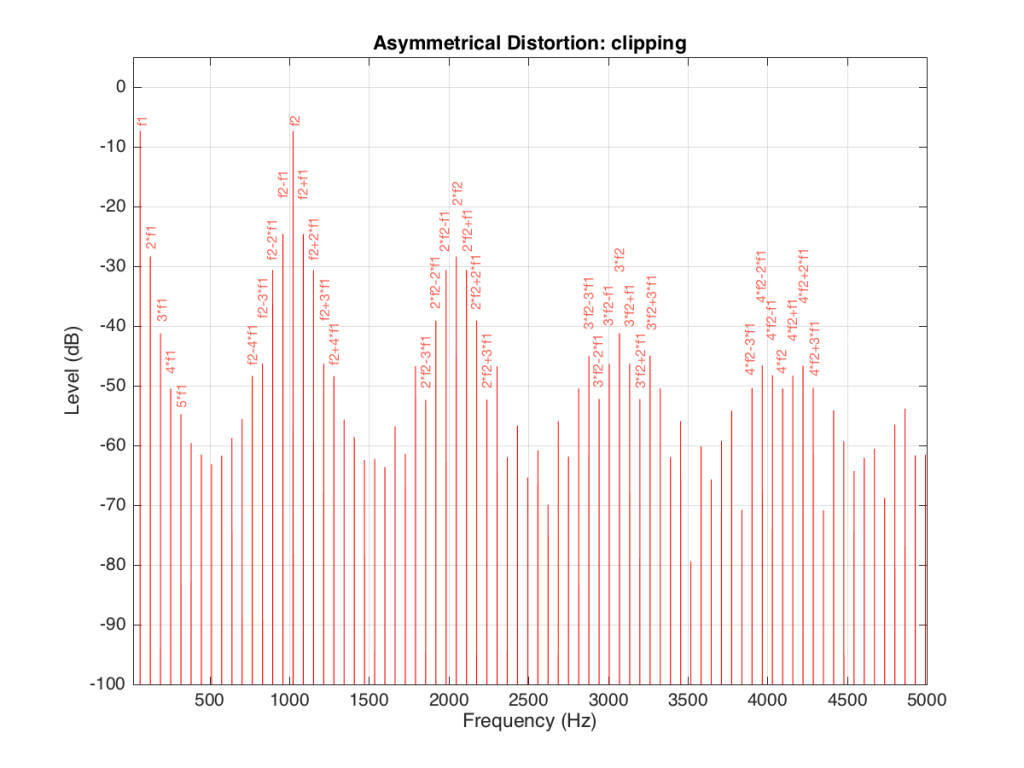
If we apply the asymmetrical clipping to the same signal, we (of course) get a different result, but it  exhibits the same characteristics, just with different values, as can be seen in Figures 15 and 16.

 

 

 

 

 

 

 

 

 

 

Wrapping up

It’s important to state once more that none of the plots I’ve shown here are based on any real loudspeaker driver. I’m using simple examples of non-linear distortion just to illustrate the effects on an audio signal. The actual behaviour of an actual loudspeaker driver will be much more complicated than this, but also much more subtle (hopefully – if not, something it probably broken…).

 

Appendix

As I mentioned at the very beginning of this posting, many of the plots in this article have an intentional error. The reason I wrote this article is to try to give you an intuitive understanding of the results of a problem with the stiffness and Bl curves of a loudspeaker driver with respect to its excursion. This means that my plots of the time domain (such as those in Figure 2) show the excursion of the driver in millimetres with respect to time. I then skip over to a magnitude response plot, pretending that the signal that comes from a driver (a measurement of the air pressure) is identical to the pattern of the driver’s excursion. This is not true. The modulation in air pressure caused by a moving loudspeaker driver are actually in phase with the acceleration of the loudspeaker driver – not its excursion. So, I skipped a step or two. However, since I wasn’t actually showing real responses from real drivers, I didn’t feel too guilty about this. Just be warned that, if you’re really digging into this, you should not directly jump from loudspeaker driver excursion to a plot of the sound pressure.