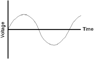
Figure 8.1: The analog waveform that we’re going to convert to digital
representation.
Once upon a time, the only way to store or transmit an audio signal was to use a change in voltage (or magnetism) that had a waveform that was analagous to the pressure waveform that was the sound itself. This analog signal (analog because the voltage wave is analogous of the pressure wave) worked well, but suffered from a number of issues, particulary the unwanted introduction of noise. Then someone came up with the great idea that those issues could be overcome if the analog wave was converted into a different way of representing it.
The first step in digitizing an analog waveform is to do basically the same thing film does to motion. When you sit and watch a movie in a cinema, it appears that you are watching a moving picture. In fact, you are watching 24 still pictures every second – but your eyes are too slow in responding to the multiple photos and therefore you get fooled into thinking that smooth motion is happening. In technical jargon, we are changing an event that happens in continuous time into one that is chopped into slices of discrete time.
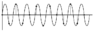
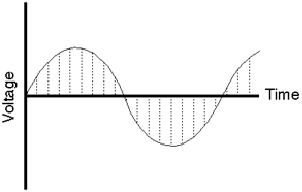
Unlike a film, where we just take successive photographs of the event to be replayed in succession later, audio uses a slightly different procedure. Here, we use a device to sample the voltage of the signal at regular intervals in time as is shown below in Figure 8.2.
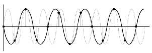
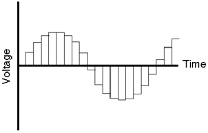
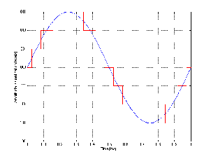
Each sample is then temporarily stored and all the information regarding what happened to the signal between samples is thrown away. The system that performs this task is what is known as a sample and hold circuit because it samples the original waveform at a given moment, and holds that level until the next time the signal is sampled as can be seen in Figure 8.3.
Our eventual goal is to represent the original signal with a string of numbers representing measurements of each sample. Consequently, the next step in the process is to actually do the measurement of each sample. Unfortunately, the “ruler” that’s used to make this measurement isn’t infinitely precise – it’s like a measuring tape marked in millimeters. Although you can make a pretty good measurement with that tape, you can’t make an accurate measurement of something that’s 4.23839 mm long. The same problem exists with our measuring system. As can be seen in Figure 8.4, it is a very rare occurance when the level of each sample from the sample and hold circuit lands exactly on one of the levels in the measuring system.
If we go back to the example of the ruler marked in millimeters being used to measure something 4.23839 mm long, the obvious response would be to round off the measurement to the nearest millimeter. That’s really the best you could do... and you wouldn’t worry too much because the worst error that you could make is about a half a millimeter. The same is true in our signal measuring circuit – it rounds the level of the sample to the nearest value it knows. This procedure of rounding the signal level is called quantization because it is changing the signal (which used to have infinite resolution) to match quanta, or discrete values. (Actually, a “quantum” according to my dictionary is “the minimum amount by which certain properties ... of a system that can change. Such properties do not, therefore, vary continuously, but in integral multiples of the relevant quantum.” [Isaacs, 1990])
Of course, we have to keep in mind that we’re creating error by just rounding off these values arbitrarily to the nearest value that fits in our system. That error is called quantization error and is perceivable in the output of the system as noise whose characteristics are dependent on the signal itself. This noise is commonly called quantization noise and we’ll come back to that later.
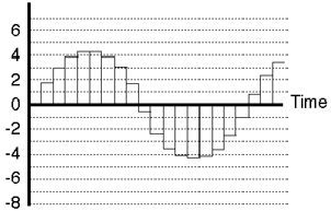
In a perfect world, we wouldn’t have to quantize the signal levels, but unfortunately, the world isn’t perfect... The next best thing is to put as many possible gradations in the system so that we have to round off as little as possible. That way we minimize the quantization error and therefore reduce the quantization noise. We’ll talk later about what this implies, but just to get a general idea to start, a CD has 65,536 possible levels that it can use when measuring the level of the signal (as compared to the system shown in Figure 8.5 where we only have 16 possible levels...)
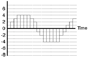
At this point, we finally have our digital signal. Looking back at Figure 8.5 as an example, we can see that the values are
0 2 3 4 4 4 4 3 2 -1 -2 -4 -4 -4 -4 -4 -2 -1 1 2 3
These values are then stored in (or transmitted by) the system as a digital representation of the original analog signal.
Now that we have all of those digits stored in our digital system, how do we turn them back into an audio signal? We start by doing the reverse of the sample and hold circuit. We feed the new circuit the string of numbers which it converts into voltages, resulting in a signal that looks just like the output of the quantization circuit (see Figure 8.5).
Now we need a small extra piece of knowledge. Compare the waveform in Figure 8.1 to the waveform in Figure 8.4. One of the biggest differences between them is that there are instantaneous changes in the slope of the wave – that is to say, the wave in Figure 8.4 has sharper corners in it, while the one if Figure 8.1 is nice and smooth. The presence of those sharp corners indicates that there are high frequency components in the signal. No high frequencies, no sharp corners.
Therefore, if we take the signal shown in Figure 8.5 and remove the high frequencies, we remove the sharp corners. This is done using a filter that blocks the high frequency information, but allows the low frequencies to pass. Generally speaking, the filter is called a low pass filter but in this specific use in digial audio it’s called a reconstruction filter (although some people call it a smoothing filter) because it helps to reconstruct (or smooth) the audio signal from the ugly staircase representation as shown in Figure 8.6.
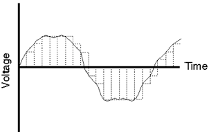
The result of the output of the reconstruction filter, shown by itself in Figure 8.7 is the output of the system. As you can see, the result is an continuous waveform (no sharp edges...). Also, you’ll note that it’s exactly the same as the analog waveform we sent into the system in the first place – well... not exactly... but keep in mind that we used an example with very bad quantization error. You’d hopefully never see anything this bad in the real world.
I remember when I was a kid, I’d watch the television show M*A*S*H every week, and every week, during the opening credits, they’d show a shot of the jeep accelerating away out of the camp. Oddly, as the jeep got going faster and faster forwards, the wheels would appear to speed up, then slow down, then stop, then start going backwards... What didn’t make sense was that the jeep was still going forwards. What causes this phenomenon, and why don’t you see it in real day-to-day life?
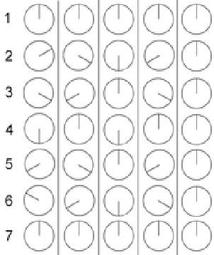
Let’s look at this by considering a wheel with only one spoke as is shown in the top left of Figure 8.8. Each column of Figure 8.8 rerpresents a different rotational speed for the wheel, each numbered row represents a frame of the movie. In the leftmost column, the wheel makes one sixth of a rotation per frame. This results in a wheel that appears to be rotating clockwise as expected. In the second column, the wheel is making one third of a rotation per frame and the resulting animation is a faster turning wheel, but still in the clockwise rotation. In the third column, the wheel is turning slightly faster, making one half of a rotation per frame. This results the the appearance of a 2-spoked wheel that is stopped.
If the wheel is turning faster than one rotation every two frames, an odd thing happens. The wheel, making more than one half of a rotation per frame, results in the appearance of the wheel turning backwards and more slowly than the actual rotation... This is a problem caused by the fact that we are slicing continuous time into discrete time, thus distorting the actual event. This result which appears to be something other than what happened is known as an alias – another representation (or name) for the truth.
The same problem exists in digital audio. If you take a look at the waveform in Figure 8.9, you can see that we have less than two samples per period of the wave. Therefore the frequency of the wave is greater than one half the sampling rate.
Figure 8.10 demonstrates that there is a second waveform with the same amplitude as the one in Figure 8.9 which could be represented by the same samples. As can be seen, this frequency is lower than the one that was recorded
The whole problem of aliasing causes two results. Firstly, we have to make sure that no frequencies above half of the sampling rate (typically called the Nyquist frequency) get into the sample and hold circuit. Secondly, we have to set the sampling rate high enough to be able to capture all the frequencies we want to hear. The second of these issues is a pretty easy one to solve: textbooks say that we can only hear frequencies up to about 20 kHz, therefore all we need to do is to make sure that our sampling rate is at least twice this value – therefore at least 40,000 samples per second.
The only problem left is to ensure that no frequencies above the Nyquist frequency get into the sample and hold circuit to begin with. This is a fairly easy task. Just before the sample and hold circuit, a low-pass filter is used to eliminate high frequency components in the audio signal. This low-pass filter, usually called an anti-aliasing filter because it prevents aliasing, cuts out all energy above the Nyquist, thus solving the problem. Of course, some people think that this creates a huge problem because it leaves out a lot of information that no one can really prove isn’t important.
There is a more detailed discussion of the issue of aliasing and antialiasing filters in Section 8.3.
If you don’t understand how to count in binary, please read Section 1.8.
As we’ll talk about a little later, we need to convert the numbers that describe the level of each sample into a binary number before storing or transmitting it. This just makes the number easier for a computer to recognize.
The reason for doing this conversion from decimal to binary is that computers – and electrical equipment in general – are happier when they only have to think about two digits. Let’s say, for example that you had to invent a system of sending numbers to someone using a flashlight. You could put a dimmer switch on the flashlight and say that, the bigger the number, the brighter the light. This would give the receiver an intuitive idea of the size of the number, but it would be extremely difficult to represent numbers accurately. On the other hand, if we used binary notation, we could say “if the light is on, that’s a 1 – if it’s off, that’s a 0” then you can just switch the light on and off for 1’s and 0’s and you send the number. (of course, you run into problems with consecutive 1’s or 0’s – but we’ll deal with that later...)
Similarly, computers use voltages to send signals around – so, if the voltage is high, we call that a 1, if it’s low, we call it 0. That way we don’t have to use 10 different voltage levels to represent the 10 digits. Therefore, in the computer world, binary is better than decimal.
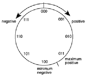
Let’s back up a bit (no pun intended...) to the discussion on binary numbers. Remember that we’re going to use those binary numbers to describe the signal level. This would not really be a problem except for the fact that the signal is what is called bipolar meaning that it has positive and negative components. We could use positive and negative binary numbers to represent this but we don’t. We typically use a system called “two’s complement.” There are really two issues here. One is that, if there’s no signal, we’d probably like the digital representation of it to go to 0 – therefore zero level in the analog signal corresponds to zeros in the digital signal. The second is, how do we represent negative numbers? One way to consider this is to use a circular plotting of the binary numbers. If we count from 0 to 7 using a 3-bit “word” we have the following:
000
001
010
011
100
101
110
111
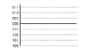
Now if we write these down in a circle starting at 12 o’clock and going clockwise as is shown in Figure 8.11, we’ll see that the value 111 winds up being adjacent to the value 000. Then, we kind of ignore what the actual numbers are and starting at 000 turn clockwise for positive values and counterclockwise for negative values. Now, we have a way of representing positive and negative values for the signal where one step above 000 is 001 and one step below 000 is 111. This seems a little odd because the numbers don’t really line up the way we’d like them as can be seen in Figure 8.12 – but does have some advantages. Particularly, digital zero corresponds to analog zero – and if there’s a 1 at the beginning of the binary word, then the signal is negative.
One issue that you may want to concern yourself here is the fact that there is one more quantization level in the negative area than there is in the positive. This is because there are an even number of quantization levels (because that number is a power of two) but one of them is dedicated to the zero level. Therefore, the system is slightly asymmetrical – so it is, in fact possible to distort the signal in the positive before you start distorting in the negative. But keep in mind that, in a typical 16-bit system we’re talking about a VERY small difference.
The fundamental difference between digital audio and analog audio is one of resolution. Analog representations of analog signals have a theoretically infinite resolution in both level and time. Digital representations of an analog sound wave are discretized (a fancy word meaning “chopped up”) into quantifiable levels in slices of time. We’ve already talked about discrete time and sampling rates a little in the previous section and we’ll elaborate more on it later, but for now, let’s concentrate on quantization of the signal level.
As we’ve already seen, a PCM-based digital audio system has a finite number of levels that can be used to specify the signal level for a particular sample on a particular channel. For example, a compact disc uses a 16-bit binary word for each sample, therefore there are a total of 65,536 (or 216) quantization levels available. However, we have to always keep in mind that we only use all of these levels if the signal has an amplitude equal to the maximum possible level in the system. If we reduce the level by a factor of 2 (in other words, a gain of -6.02 dB) we are using one fewer bit’s worth of quantization levels to measure the signal. The lower the amplitude of the signal, the fewer quantization levels that we can use until, if we keep attenuating the signal, we arrive at a situation where the amplitude of the signal is the level of 1 Least Significant Bit (or LSB).
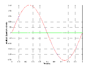
Let’s look at an example. Figure 8.13 shows a single cycle of a sine wave plotted with a pretty high degree of resolution (well... high enough for the purposes of this discussion).
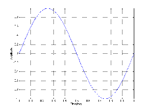
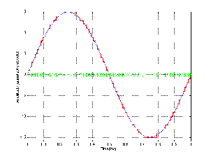
Let’s say that this signal is converted into a PCM digital representation using a converter that has 3 bits of resolution – therefore there are a total of 8 different levels that can be used to describe the level of the signal. In a two’s complement system, this means we have the zero line with 3 levels above it and 4 below. If the signal in Figure 8.13 is aligned in level so that its positive peak is the same as the maximum possible level in the PCM digital representation, then the resulting digital signal will look like the one shown in Figure 8.14.
Not surprisingly, the digital representation isn’t exactly the same as the original sine wave. As we’ve already seen in the previous section, the cost of quantization is the introduction of errors in the measurement. However, let’s look at exactly how much error is introduced and what it looks like.
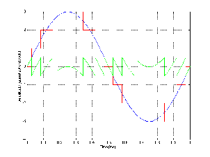
This error is the difference between what we put into the system and what comes out of it, so we can see this difference by subtracting the red waveform in Figure 8.14 from the blue waveform. The result of this is shown in Figure 8.15.
There are a couple of characteristics of this error that we should discuss. Firstly, because the sine wave repeats itself, the error signal will be periodic. Also, the period of this complex waveform will be identical to the original sine wave – therefore it will be comprised of harmonics of the original signal. Secondly, notice that the maximum quantization error that we introduce is one half of 1 LSB. The significant thing to note about this is its relationship to the signal amplitude. The quantization error will never be greater than one half of an LSB, so the more quantization levels we have (in other words, the more LSB’s that equal 1 MSB), the louder we can make the signal we want to hear relative to the error that we don’t want to hear. See Figures 8.14 through ?? for a graphic illustration of this concept.
As is evident from Figures 8.16, 8.17 and 8.18, the greater the number of bits that we have available to describe the instantaneous signal level, the lower the apparent level of the quantization error. I use the word “apparent” here in a strange way – no matter how many bits you have, the quantization error will be a signal that has a peak amplitude of one half of an LSB in the worst case. So, if we’re thinking in terms of LSB’s – then the amplitude of the quantization error is the same no matter what your resolution. However, that’s not the way we normally think – typically we think in terms of our signal level, so, relative to that signal, the higher the number of available quantization levels, the lower the amplitude of the quantization error.
Given that a CD has 65,536 quantization levels available to us, do we really care about this error? The answer is “yes” – for two reasons:
Remember as well that this can happen to one quiet signal in the presence of a louder one. For example, if you take a recording of a plucked guitar string, the signal-to-error ratio decreases as the note decays. If you pluck another string of the guitar while the first one is still decaying, then you will still have a large error on the decay of the first note, despite the fact that the second note has a high amplitude. Another example of this problem is when you have reverberation decaying under more recent notes coming from the instrument(s).
Distortion is something different. Distortion, like noise, is typically comprised entirely of unwanted material (I’m not talking about guitar distortion effects or the distortion of a vintage microphone here...). Unlike noise, however, distortion products modulate with the signal. Consequently the brain thinks that this is important material because it’s trackable, and therefore you’re always paying attention. This is why it’s much more difficult to ignore distortion than noise. Unfortunately, quantization error produces distortion – not noise.
Luckily, however, we can make a cute little trade. It turns out that we can effectively eliminate quantization error simply by adding noise called dither to our signal as is shown in Figure 8.19. It seems counterproductive to fix a problem by adding noise – but we have to consider that what we’re esentially doing is to make a trade – distortion for noise. By adding dither to the audio signal with a level that is approximately one half the level of the LSB, we generate an audible, but very low-level constant noise that effectively eliminates the program-dependent noise (distortion) that results from low-level signals.
Notice that I used the word “effectively” at the beginning of the last paragraph. In fact, we are not eliminating the quantization error. By adding dither to the signal before quantizing it, we are randomizing the error, therefore changing it from a program-dependent distortion into a constant noise floor. The advantage of doing this is that, although we have added noise to our final signal, it is constant, and therefore not readily trackable by our brains. Therefore, we ignore it more easily. In fact, by adding noise at the level of something on the order of 1 LSB we are applying the quantization error to the noise, consequently, the error is random.
So far, all I have said is that we add “noise” to the signal, but I have not said what kind of noise – is it white, pink, or some other colour? People who deal with dither typically don’t use these types of terms to describe the noise – they talk about probability density functions or PDF instead. When we add dither to a signal before quantizing it, we are adding a random number that has a value that will be within a predictable range. The range has to be controlled, otherwise the level of the noise would be unnecessarily high and therefore too audible, or too low, and therefore ineffective.
If you don’t already understand the concept of a probability distribution function, it’s explained in Section 4.16.
There are three typical dither PDF’s used in PCM digital audio, RPDF, TPDF (triangular PDF) and Gaussian PDF. We’ll only look at the first two.
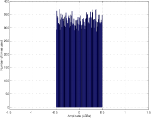
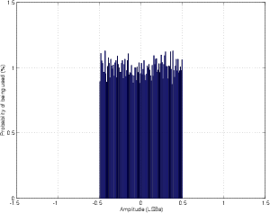
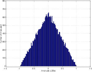
Before we get into the details of what dither really does, let’s look at a couple of examples of its effects, shown in Figures 8.20 to 8.23.
RPDF dither has an equal probability of being any level between -0.5 LSB and 0,5 LSB. Remember that the dither signal is added before the quantization, so it can be a voltage level less than whatever voltage is equivalent to 1 LSB.
If you’re using MATLAB and you consider an LSB to be an integer value (in other words, 1 LSB = 1, and therefore a CD signal ranges from -32,768 to 32,767) then you can create one channel of RPDF dither using the command RAND(1, n) - 0.5 where n is the length of the signal in samples.
TPDF dither has the highest probability of being 0, and a 0 probability of being either less than -1 LSB or more than 1 LSB. This can be made by adding two random numbers, each with an RPDF together. Using MATLAB, this is most easily done using the command RAND(1, n) - RAND(1, n) where n is the length of the dither signal, in samples. The reason they’re subtracted here is to produce a TPDF that ranges from -1 to 1 LSB.
So, for example if you wanted to make a 1-second long 997 Hz sine wave at -20 dB FS with RPDF or TPDF dither quantized for 16 bits with a sampling rate of 44.1 kHz, you could use the following MATLAB code.
Let’s look at the results of three options: no dither, RPDF dither and TPDF dither. Figure 8.31 shows a frequency analysis of 4 signals (from top to bottom): (1) a 64-bit 1 kHz sine wave, (2) an 8-bit quantized version of the sine wave without dither added, (3) an 8-bit quantized version with RPDF added and (4) an 8-bit quantized version with TPDF added.
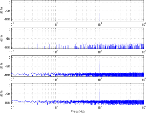
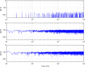
One of the important things to notice here is that, although both types of dither raised the overall noise floor of the signal, the resulting artifacts are wide-band noise, rather than spikes showing up at harmonic intervals as can be seen in the no-dither plot. If we were to look at the artifacts without the original 1 kHz sine wave, we get a plot as shown in Figure 8.32.
So, at this point, you should be asking what the difference is between RPDF and TPDF dither, since both of their FFT outputs look pretty much the same. In fact, for the example I gave, where the signal was a steady-state sine wave, the results are pretty much the same. However, if we were to use the two types of dither in real-world examples, where the signals were musical examples instead of sine waves, then you would hear the difference almost immediately.
If we use RPDF dither, and listen to a sine wave quantized using only 2 or 3 bits, you’ll hear a lot of noise (the quantized dither) and the sine tone. If we used TPDF dither for the same signal and the same bit depth, we would hear a different-sounding noise and the sine tone. So far, they’re still the same. However, if we did the same experiment with music, we’d hear two very different things. You would notice that the noise floor with the RPDF dither was modulating with the signal strength. The higher the signal level, the higher the noise floor, up to a maximum, after which the noise stops getting louder and the signal just goes up and up. With TPDF dither, the noise floor remains at a constant level, regardless of the signal strength.
One way to understand the effect of dither on a signal is to see its effects on photographs. In order to do this, I started with a colour photograph that I took and converted to an 8-bit grayscale representation. This means there are 28 or 256 different possible levels of gray to choose from for each pixel. If 0 is assigned to a pixel, then it is completely black, if it’s 255, then it’s completely white. A value between 0 and 255 will be some shade of gray between the two. (You may be curious to note that, when people talk about “24-bit colour,” this actually means that you have 8 bits for representing each of the three component colours in the photo – red, green and blue. 8 bits x 3 colours = 24 bits.)
The original 8-bit grayscale photograph that was used for the rest of the examples in this section is shown in Figure 8.33.
Let’s begin by taking the original photograph in Figure 8.33 and rounding off the values of gray with fewer and fewer levels from which to choose. In other words, we are reducing the number of bits that are available to describe the gray levels. If we take this procedure to an extreme, we end at only two levels of “gray” being black and white.
Some examples of this for various bit depths are shown in Figures 8.34 to 8.37. The obvious effect to look for in the various levels of bit depth reduction is the increasing loss of detail. Smooth gradients that go from light to dark are converted to monochromatic patches.
If we add RPDF dither to the photo before re-quantizing at our new bit depth, we get a different effect, shown in Figures 8.39 to 8.42.
The dither signal itself is shown in Figure 8.38, however, you should be a little careful when you’re looking at that figure. The dither shown in Figure 8.38 is scaled (amplified) so that it ranges from black to white. This was done to make it easier to see. In reality, when the dither signal is added to the original photo, it will range from gray to a different gray.
This time, when looking at the RPDF dithered, quantized versions of the photo, notice that, to some extent the monochromatic patches still exist, however the transition between those patches is smoothed, allowing us to see more details than was possible in the non-dithered, quantized equivalents. Interestingly, it is even possible to detect some details in the black and white (1-bit) version, shown in Figure 8.42. This is because your brain is very good at finding (or tracking) a pattern in the noise.
Finally, we’ll do the same thing using TPDF dither, shown in Figure 8.43. If you compare this Figure with the RPDF equivalent in Figure 8.38, you’ll may notice that the TPDF version looks a little “smoother.” This is due to the probability density function of the gray levels. In the RPDF version, a pixel has an equal probability of being any level of gray. Therefore, you can just as easily find a dark pixel next to a light pixel as you can find two similar pixels side-by-side. In the TPDF version, a pixel is most likely to have a middle value of gray, and it’s very unlikely for a pixel to be very light or very dark. Therefore, if you look, pixel by pixel, you’ll see more mid-grays than anything else.
Figures 8.44 to 8.47 show the same original photo, added to TPDF dither and quantized at different bit depths. You’ll see in these photos that the photos look a little more noisy than the ones in the RPDF examples, however, you don’t lose the details in monochromatic patches in these examples. This is even true for the black and white (1-bit) example in Figure 8.47. If you zoom into this photo on your screen, you will see that the pixels are either black or white – none of them are gray. However, if you zoom out, you can easily see most of the details on the front of the building. Admittedly, you do lose some fine details such as the time on the clock due to the fact that these fine details in the photo (the signal) are below the noise floor of the image.
ADD A LINK TO A WEB PAGE HERE
I once attended a seminar on digital audio measurements given by Julian Dunn. At lunch, I sat at a table of about 12 people, and one of the other participants asked me the simple question “what do you think about dither?” I responded that I thought it was a good idea1 . Then the question was re-phrased – “yes, but when do you use it?” The answer is actually pretty simple – you use dither whenever you have to re-quantize a signal. Typically, we do DSP on our audio signals using word lengths much greater than the original sample, or the resulting output. For example, we typically record at 16 or 24 bits (with dither built into the ADC’s), and the output is usually at one of these two bit depths as well. However, most DSP (like equalization, compression, mixing and reverberation) happens with an accuracy of 32 bits (although there are some devices such as those from Eventide that run at 64-bit internally). So, a 16-bit signal comes into your mixer, it does math with an accuracy of 32 bits, and then you have to get out to a 16-bit output. The process of converting the 32-bit signal into a 16-bit signal must include dither.
Remember, if you are quantizing (or re-quantizing), then you dither – every time.
Back in Section 8.1.3, we looked very briefly at the problem of aliasing, but now we have to dig a little deeper to see more specifically what it does and how to avoid it.
As we have already seen, aliasing is an artifact of chopping continuous events into discrete time. It can be seen in film when cars go forwards but their wheels go backwards. It happens under fluorescent or strobe lights that prevent us from seeing intermediate motion. Also, if we’re not careful, it happens in digital audio.
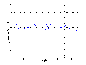
Let’s begin by looking at a simple example: we’ll look at a single sampling rate and what it does to various sine waves from analog input to analog output from the digital system.
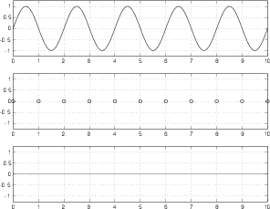
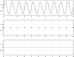
Figure 8.62 shows three plots, the top is an analog signal that has a frequency of one tenth the sampling rate. This frequency can be deduced by counting the number of samples that are used to represent it, shown in the middle plot. The bottom plot shows the end result of converting the samples in the middle plot back to the analog domain. Note here that we’re ignoring any quantization effects.
As you can see by comparing the top and bottom plots in Figure 8.62, the output is a pretty darned good reproduction of the original input. So far so good.
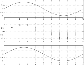
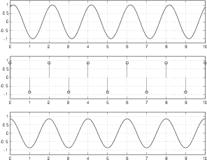
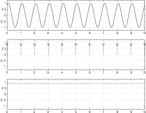
Figure 8.63 shows a similar set of plots to those shown in Figure 8.62, however, now the analog signal that we’re digitizing is a sinusoidal wave with a frequency of 0.4 of the sampling rate (because there are 4 cycles of the waveform in 10 sampling periods – 4/10 = 0.4).
As can be seen in comparing the top and bottom plots in Figure 8.63, the system is still working well.
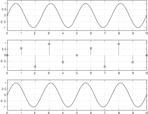
Figure 8.64 shows the signal frequency where things suddenly fall apart. In this plot, the sinusoidal analog signal is at the Nyquist frequency – one half the sampling rate (5 cycles in 10 sampling periods). As can be seen in the middle plot, the samples used to represent the signal measure the amplitude of the waveform at the same place on the wave on every cycle. The result is that all samples have the same value, and therefore produce a DC output instead of the sinusoidal wave we put into the converter.
Figure 8.64 is a special case – I carefully lined up the analog signal and the samples so that the samples are measuring the signal at its zero crossings to prove that there can be instances where the system breaks down. However, if I had lined the two up so that the samples were measuring the peaks of the analog signal, we would get a sinusoidal output. The point here is that, at one half the sampling rate, the system is unreliable. The output analog signal will have the correct frequency most of the time (when the samples don’t line up with the zero crossings in the input signal) but it will have an amplitude and phase that is dependent on the phase relationship between the analog input and the samples. An example of this problem is shown in Figure 8.65.
Okay, so we know that a PCM system will break down when the input signal is one-half the sampling rate, but what happens if the input signal has an even higher frequency? Take a look at Figure 8.66. Here we have a sinusoidal input signal with a frequency of 0.6 of the sampling rate. The samples measure the signal at the sampling period and produce an interesting output. We can see in the bottom plot that the resulting output signal does not have the same frequency as the input. In fact, it has a frequency of 0.4 of the sampling rate. These is an interesting point to discuss.
We input a signal with a frequency that is 0.6 of the sampling rate. The output has a frequency that is 0.4 of the sampling rate. We could jump to a conclusion here and say that, if the input signal is higher than the Nyquist frequency, the output’s frequency will be equal to the input frequency mirrored across the Nyquist frequency. In fact, this is a safe conclusion to jump to, because it’s true.
If we want to express this as an equation, it would look something like Equation 8.1
 | (8.1) |
Note that Equation 8.1 is somewhat oversimplified in that it only is true when fout is between the Nyquist frequency and the sampling rate. We’ll look at a more general equation to cover all cases later in the section.
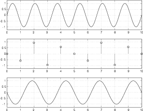
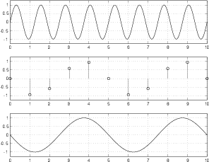
Figure 8.67 shows an input with a frequency of 0.8 of the sampling rate. The output is 0.2
When the input signal reaches the sampling rate itself, we get another special case. As can be seen in Figure 8.68, the samples measure the input at the same point on every cycle. The result is a DC output. In the specific case of Figure 8.68, I lined things up so that the samples measure the zero-crossings, so the output is silence.
If the input signal is the same frequency as the sampling frequency, but they doesn’t happen to line up nicely, then we get a DC output from the system as is shown in Figure 8.69. This DC output can vary from the minimum value to the maximum value of the input signal, and is dependent on the phase relationship between the input signal and the sampling time.
NOT YET WRITTEN
So far, we have only looked at some of the basic concepts of converting an analog signal to a digital representation of it, and back again. (Okay, okay... admittedly, nothing in this book will get past basic concepts. If you are planning on knowing enough to build a converter, then you should probably go read a different book...) Now let’s look a little deeper into some aspects that you’ll need to know.
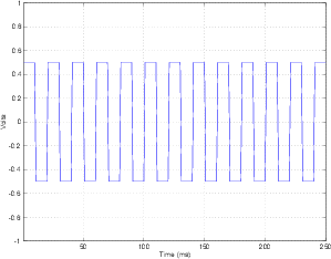
Take a square wave with a peak voltage of 0.5 V, a 50% duty cycle and no DC offset like the one shown in Figure 8.70.
Take a window of time more than one cycle long, and average all of the voltages in that window. Since the square wave has a 50% duty cycle, it’s on a high voltage as often as it’s on a low voltage. That means that, if the averaging window is long enough, its output will be 0 V.
Let’s keep the amplitude of the square wave and change its duty cycle to 70% as is shown in Figure 8.71.
Now the output of the averaging will be 0.2 V. This is because the square wave is asymmetrical and is on a high voltage longer than it’s on a low voltage within the averaging window.
The moral of this story is that, to control the output of the averaging window, all we have to do is to change the duty cycle of the square wave.
Something interesting has happened here... We have taken a signal that has only two “states” – a high voltage and a low voltage, and, by changing only its duty cycle, we can create any output voltage between those two voltages simply by doing a time average of the signal. This is the principal behind a 1-bit digital signal. We can consider the square wave to be a digital signal consisting of 0’s (the low’s) and 1’s (the high’s), and the output of the averaging window to be the analog signal.
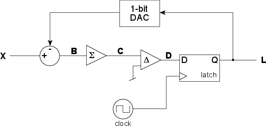
So, how do we create that digital signal in the first place? Take a look at the block diagram in Figure 8.72.
To begin with, let’s look at what each of the components in the circuit do.
The circle at the left of the figure has two inputs and one output. The voltage signal coming in the top is subtracted from the voltage signal coming in the left and the result is sent to the output. This is essentially the same as a differential amplifier described in Section 2.10.9.
The triangle with the Σ symbol in it is what’s called an integrator. It keeps track of all of its input and continuously adds it to what came before. Think of it like a tank with a hose running into it. The reason the integrator doesn’t overload is that the input signal is usually going positive and negative. When the input is positive, the output of the integrator keeps creeping up, when the input is negative, the output of the integrator keeps creeping down. Note that in most books, this component will be marked with a symbol like ∫ (because that’s the sign for integration, and the device is an integrator). I’m using a Σ to represent the device because, although it’s an integrator, the name of the whole device has the word “Sigma” in it.
The triangle with the Δ symbol in it is called a comparator. It compares the voltage levels of its two inputs and gives an output that tells you which of the inputs is higher than the other. Notice that the lower input is connected to ground, therefore it is kept constant at 0 V. When the other input is higher than 0 V, the output of the comparator is high (let’s say, 1 V). When the other input is lower than 0 V, the output of the comparator is low (let’s say, -1 V).
The rectangle on the right is called a latch. It has two inputs, one labeled with a “D” and the other with a triangle, and one output labeled “Q.” You send a signal into the D input that can be either high or low (in fact, in our case, it’s always changing between high and low, but we never know when). The signal coming in the triangle input is a clock signal that tells the latch to look at the other input and make the output the same, and to hold that value until the next clock tick. Essentially, the latch ignores the “D” input until a clock pulse comes in. When the clock ticks it grabs the value at the “D” input and outputs that value. Then it holds the output at that value until the clock ticks again.
The clock at the bottom of the block diagram is just a square wave generator. A “tick” of the clock is the instant when the square wave changes from a low to a high voltage.
Finally, the rectangle at the top is a 1-bit digital to analog converter. If the input of the DAC is a high voltage, then it outputs a high voltage. If the input of the DAC is a low voltage, then it outputs a low voltage. (Sounds complicated... I know...) In our case, if the input voltage is 1 V, then the output is 1 V, if the input voltage is 0 V, then the output is -1 V.
Let’s take a simple example where we input silence into the converter, keeping it at a constant 0 V. We’ll also assume that the output of the DAC is -1. Therefore, the signal at point “B” in the schematic is 1 V. The output of the integrator (at point “C”) starts creeping up above 0, getting higher and higher as time passes. The comparator sees an input signal higher than 0 V and makes the output at point “D” high. When the clock ticks, the output of the latch is high. This makes the signal at point “L” high and the output of the DAC high as well.
This makes the signal at “B” go low (because we’re now subtracting a high value from the 0 V input) which pulls the output of the integrator down. Eventually, the signal at “C” reaches 0 V or lower, and the output of the comparator goes low. The clock ticks, and the latch grabs the low input and sends it out the output. This makes the DAC go low, and the whole process repeats itself.
The result of this is that the signal at point “L” in the circuit (the output of the latch, which is also the output of the ADC) is a square wave with a 50% duty cycle.
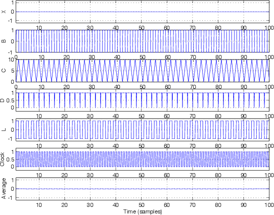
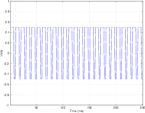
Let’s take this signal at point “L” in the schematic and average it with a window of 10 samples. The output of that averaging is plotted at the bottom of Figure 8.73. Notice that that signal is remarkably similar to the input signal “X.”
What happens if the input signal is a sine wave? Take a look at Figure 8.74. I won’t bother going through the signal step by step...
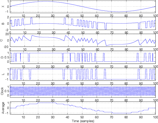
You’ll notice that the averaging output plotted at the bottom of Figure 8.74, again, looks remarkably similar, but not identical to the input signal at the top of the figure. However, you may also notice that the signal is the sine wave with some high frequency noise screwing up the signal. Therefore, in order to fix this, all we need to do is to low-pass filter this signal to smooth things out and get our original sine wave back. In fact, one way to average signals is to just put them through a low-pass filter. Therefore, (and this is one of the cool things about a ΔΣ system) the entire DAC can be just a low-pass filter. (Remember this point. It will come in very handy when we start talking about Class-D amplifiers.)
What we have is a digital representation (signal “L” ) of the analog input (signal “X”) using only 1 bit instead of the multiple bits that we needed for PCM conversion described in Section 8.1. So, the advantage of this system is that we have only 1 bit instead of a lot of bits to represent the signal. The big disadvantage is that we have to have a much higher sampling rate in this system. Typically we see sampling rates on the order of 64 times the highest analog signal frequency component (as opposed to 2 times, as we saw in PCM conversion).
We saw in the previous section that using a 1-bit converter does indeed distort the signal, just like a multi-bit PCM converter. In the case of the PCM converter, we saw that, for a sinusoidal input signal, the noise that the conversion process generated was periodic and signal dependent, therefore it wasn’t really noise, but distortion. The answer to this problem was to add noise (dither) to randomize the error and produce white noise that is independent of the input signal.
The behaviour of a ΔΣ conversion process is a little different. In the example presented in Figure 8.74, the sampling rate was 100 times the frequency of the signal we were sampling. In addition, the averaging window we used to get the analog back from the digital representation was only 10 samples long. The result of these two was a pretty badly distorted output, however, this should not bias you against ΔΣ conversion. Typically, the sampling rate will be much, much higher than this, and the averaging window will be much, much, much longer.
Let’s just consider the second of these two for a moment. The longer the window length in the averaging process, the less small “bumps” in the digital signal will affect the output. So, in order to smooth the analog output from our ΔΣ DAC, we just need to make sure that we have a very long time constant in our averaging process. Of course, it doesn’t help to have a long averaging window if it doesn’t contain a lot of samples, so we’ll also want a very high sampling rate. The higher the sampling rate and the longer the averaging window, the less distortion we’ll have in the final output signal.
Let’s think of this in the opposite direction... The higher the frequency of our signal, the more distortion (or noise) will be added to it by the ΔΣ converter. In fact, we get a 6 dB rise per octave in the amplitude of the unwanted (noise) signal, eventually reaching a frequency where the noise is the same amplitude as the signal that we’re encoding, therefore having a SNR of 0 dB. This is bad.
However, there is one saving grace... The frequency where the SNR of a ΔΣ converter is 0 dB is at the Nyquist Frequency – one half the sampling rate. Since we’ve already decided to make our sampling rate very, very high, this means that the resulting noise will be low, right? Maybe...
Let’s take a pretend ΔΣ system with a sampling rate of 11.2896 MHz (44.1 kHz times 256) We know that the SNR of this system is 0 dB when the input signal is at 5.6448 MHz, and it increases by 6.02 dB every time we drop an octave. Therefore, at a 22,050 kHz, the SNR of our system is 54 dB. This is not bad, but it’s not nearly as good as even a 16-bit system. As we get lower and lower in frequency, our SNR gets better and better. At 1378 Hz, it’s 78 dB. At 21 Hz, it’s 114 dB. (Remember for the sake of comparison that a 16-bit PCM converter has a wide-band SNR of 93 dB, and a 24-bit converter has a SNR of 141 dB.)
Okay, so far, our fancy ΔΣ isn’t looking so hot... but wait... what we’ve been talking about up to now is something called a first-order ΔΣ modulator. (It’s called a first-order modulator because it contains only one integrator.) It is well-known by people who build converters that a first-order ΔΣ produces a quantization error that is highly correlated with the signal[Pohlmann, 1991].
How do we get around this problem? We do it by being clever. We cannot eliminate noise, however, we know that the noise is caused by error which in turn is caused by quantizing the signal. So, if we can calculate what the error is, then we can predict (in fact, we’ll know) what the noise will be. We can’t eliminate the noise, but we can move it. Since we’ve already seen that we are pretty deaf at high frequencies, what is typically done is to push the noise caused by the error up into the higher frequency bands, therefore reducing the noise level in the lower bands, where we’re paying attention to what’s going on. A nice benefit to the ΔΣ system is that, since the sampling rate is so high (because it has to be...) we can push the noise up into the extremely high frequencies, out of range of our hearing where we really don’t care about it at all.
We’ll talk more about this concept called noise shaping in a later chapter.
Back in the old days (the early 90’s, to be precise), if you bought a DAT machine (Digital Audio Tape – for you folks that are younger than me...), it claimed it had 16-bit ADC’s and DAC’s. This was ostensibly true – the DAT format can store 16 bits, so 16 bits came out of the ADC and 16 bits went into the DAC. Whether or not these bits (in particular the bottom ones...) were anything close to being accurate is debatable, but we’ll say that they were for the purposes of this book.
Back in those days, the digital brains in the ADC and DAC weren’t as powerful as they are in modern converters. They could spit out 16 bits at up to 48 kHz, but that was right at the edge of their capabilities. Consequently, the ADC was preceded by an antialiasing filter (which we already know is absolutely necessary) that was implemented in the analog domain. This means that a very expensive analog circuit was stuck in front of the ADC to ensure that nothing above about 20 kHz got into the input of the converter. Of course, we audio engineers insisted that the system be laser-flat up to 20 kHz (because we’re geeks...) so the design and construction of these filters was not a trivial matter. In good gear, they were really complicated and expensive. In cheaper gear, they weren’t good enough (in fact, you can easily tell a recording made with one of the consumer DAT’s that everyone was using (no names... but it was black and it had a bigger brother (in bluish-gray) that used the same transport and an auxiliary converter section...) by the constant ringing of the anti-aliasing filter in the high end.)
Once DSP chips got faster, the manufacturers realized that they could save money by doing analog-to-digital conversion as a two-step process. Lucky for us, this also made the quality of the process better in addition to being cheaper. In the first step, the signal is converted using a ΔΣ converter. The anti-aliasing filter in front of this is analog, but since the sampling rate is very high, it could have a very low order and therefore a gentle roll-off and therefore no ringing. The output of this ΔΣ converter was subsequently fed into a digitally-implemented low-pass filter and a system for converting the ΔΣ signal into a PCM output. This all happens inside the ADC itself, and is now the standard system that has been used by pretty much everyone for about 10 years or so.
Not only does this save money (because the filter is implemented digitally instead of with a bunch of components) but it’s more stable (over time, and from device to device) and it sounds better (because it’s easier to implement better filters for a little cash in the digital domain).
INSERT A BLOCK DIAGRAM HERE
If we want to send a digital (we’ll assume that this, in turn means “binary”) signal across a wire, the simplest way to do it is to have a ground reference and some other DC voltage (5 V is good...) and we’ll call one “0” (being denoted by ground) and the other “1” (5 V). If we then know WHEN to look at the electrical signal on the wire (this timing can be determined by a clock...), we can know whether we’re receiving a 0 or 1. This system would work – in fact it does, but it has some inherent problems which would prevent us from using it as a method of transmitting digital audio signals around the real world.
Back in the early 1980’s a committee was formed by the Audio Engineering Society to decide on a standard protocol for transmitting digital audio. For the most part, they got it right... They decided at the outset that they wanted a system that had some specific characteristics and, consequently some resulting implications :
The protocol should use the cables, connectors and jackfields already existing in the recording studios. In addition, it should withstand transmission through existing analog equipment. The implications of this second specification are:
The result was the AES/EBU protocol (also known as IEC-958 Type 1). It’s a bi-phase mark coding protocol which fulfills all of the above requirements. “What’s a bi-phase mark coding protocol?” I hear you cry... Well what that means is that, rather than using two discrete voltages to denote 1 and 0, the distinction is made by voltage transitions.
In order to transmit a single bit down a wire, the AES/EBU system carves it into two “cells.” If the cells are the same voltage, then the bit is a 0 : if the cells are different voltages, then the bit is a 1. In other words, if there is a transition between the cells, the bit is a 1. If there is no transition, the bit is a 0. This is illustrated in Figure 8.75.
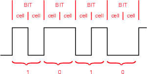
The peak-peak level of this signal is between 2 V and 7 V. The source impedance is 150Ω (this is the impedance between pins 2 and 3 on the XLR connector).
Note that there is no need for a 0 V reference in this system. The AES/EBU receiver only looks at whether there is a transition between the cells – it doesn’t care what the voltage is – only whether it’s changed.
The only thing we’ve left out is the “self-clocking” part. This is accomplished by a circuit known as a Phase-Locked Loop (or PLL to its friends...). This circuit creates a clock using an oscillator which derives its frequency from the transistion rate of the voltage it receives. The AES/EBU signal is sent into the PLL which begins in a “capture” mode. This is a wide-angle view where the circuit tries to get a basic idea of what the frequency of the incoming signal is. Once that’s accomplished, it moves into “pull-in” mode where it locks on the frequency and stays there. This PLL then becomes the clock which is used by the receiving device’s internal things (like buffers and ADC’s).
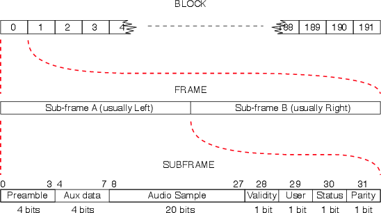
AES/EBU data is send in Blocks which are comprised of 192 Frames. Each frame contains 2 Sub-Frames, each of which contains 32 bits of information. The layout goes like this :
The information in the sub-frame can be broken into two categories, the channel code and the source code, each of which comprises various pieces of information.
| Code | Channel Code | Source Code |
| Contents | Preamble | Audio Sample |
| Parity Bit | Auxiliary data | |
| Validity Bit | ||
| User Bit | ||
| Status Bit | ||
This is information regarding the transmission itself – data that keeps the machines talking to each other. It consists of 5 bits making up the preamble (or sync code) and the parity bit.
Preamble (also known as the Sync Code)
These are 4 bits which tell the receiving device that the trasmission is at the beginning of a block or a subframe (and which subframe it is...) Different specific codes tell the receiver what’s going on as is shown in Figure 8.77.
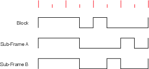
Note that these codes violate the bi-phase mark protocol (because there is no transition at the beinning of the second bit.) but they do not violate the no-DC rule (because there is the same amount of high voltage as low voltage).
Note as well, that these are sometimes called the X, Y, and Z preambles. An X preamble indicates that the sub-frame is an audio sample for the Left. A Y preamble indicates that the sub-frame is an audio sample for the right. A Z preamble indicates the start of a block.
This is a single bit which ensures that all of the preambles are in phase. It doesn’t matter to the receiving device whether the preambles start by going up in voltage or down (I drew the above examples as if they are all going up...) but all of the preambles must go the same way. The partity bit is chosen to be a 1 or 0 to ensure that the next preamble will be headed in the right direction.
This is the information that we’re trying to transmit. It uses the other 27 bits of the sub-frame comprising the audio sample (20 bits), the auxiliary data (4 bits), the validity bit (1 bit), the user bit (1 bit) and the status bit (1 bit).
This is the sample itself. It has a maximum of 20 bits, with the Least Significant Bit sent first.
This is 4 bits which can be used for anything. These days it’s usually used for 4 extra bits to be attached to the audio sample – bringing the resolution of the sample up to 24 bits.
This is simply a flag which tells the receiving device whether the data is valid or not. If the bit is a 1, then the data is non-valid. A 0 indicates that the data is valid. Some manufacturers use this bit to indicate whether the signal is PCM Audio (and can therefore be sent straight to a DAC) or something else (such as an AC-3 or DTS encoded signal). Then again, other manufacturers think that an encoded signal is valid...
This is a single bit which can be used for anything the user or manufacturer wants (such as time code, for example).
For example, a number of user bits from successive sub-frames can be strung together to make a single word. Usually this is done by collecting all 384 user bits (one from each sub frame) for each channel in a block. If you then put these together, you get 48 bytes of information in each channel.
Typically, the end user in a recording studio doesn’t have direct access to how these bits should be used. However, if you have a DAT machine, for example, that is able to send time code information on its digital output, then you’re using your user bits.
This is a single-bit flag which can be used for a number of things such as :
This information is arranged in a similar method to that described for the User Bits. 192 status bits are collected per channel per block. Therefore, you have 192 bits for the A channel (left) and 192 for the B channel (right). If you string these all together, then you have 24 bytes of information in each channel. The AES/EBU standard dictates what information goes where in this list of bytes. This is shown in the diagram in Figure ??
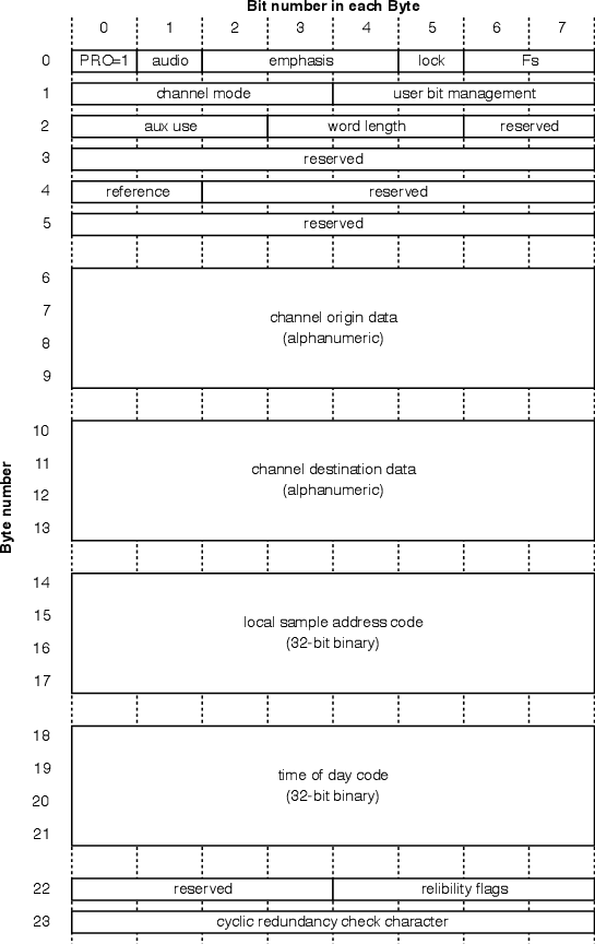
For specific information regarding exactly what messages are given by what arrangement of bits, see [Sanchez and Taylor, 1998] available as Application Note AN22 from www.crystal.com.
The AES/EBU standard (IEC 958 Type 1) was set in 1985.
The maximum cable run is about 300 m balanced using XLR connectors. If the signal is unbalanced (using a transformer, for example) and sent using a coaxial cable, the maximum cable run becomes about 1 km.
If the Sampling Rate is 44.1 kHz, 1 frame takes 22.7 μsec. to transmit (the same as the time between samples)
If the Sampling Rate is 48 kHz, 1 frame takes 20.8 μsec. to transmit
At 44.1 kHz, the bit rate is 2.822 Mbit/s
At 48 kHz, the bit rate is 3.072 Mbit/s
Just for reference (or possibly just for interest), this means that 1/4 wavelength of the cell in AES/EBU is about 19 m on a wire.
S/PDIF was developed by Sony and Philips (hence the S/P) before AES/EBU. It uses a single unbalanced coaxial wire to transmit 2 channels of digital audio and is specified in IEC 958 Type 2. The Source Code is identical to AES/EBU with the exception of the channel status bit which is used as a copy prohibit flag.
Some points :
The connectors used are RCA phono with a coaxial cable
The voltage alternates between 0V and 1V ±20% (note that this is not independent of the ground as in AES/EBU)
The source impedance is 75Ω
S/PDIF has better RF noise immunity than AES/EBU because of the coax cable (please don’t ask me to explain why... the answer will be “dunno... too dumb...”)
It can be sent as an analog “video” signal through exisiting video equipment
Signal loss will be about -0.75 dB / 35 m in video cable
Two synchronous devices have a single clock source and there is no delay between them. For example, the left windshield wiper on your car is synchronous with the right windshield wiper.
Two asynchronous devices have absolutely no relation to each other. They are free-running with separate clocks. For example, your windshield wipers are asynchronous with the snare drum playing on your car radio.
Two isochronous devices have the same clock but are separated by a fixed propogation delay. They have a phase difference but that difference remains constant.
See the next section.
Sanchez, C. and Taylor, R. (1998) Overview of Digital Audio Interface Data Structures. Application Note AN22REV2, Cirrus Logic Inc. (available at http://www.crystal.com)
Go and make a movie using a movie camera that runs at 24 frames per second. Then, play back the movie at 30 fps. Things in the movie will move faster than they did in real life because the frame rate has speeded up. This might be a neat effect, but it doesn’t reflect reality. The point so far is that, in order to get out what you put in, a film must be played back at the same frame rate at which is was recorded.
Similarly, when an audio signal is recorded on a digital recording system, it must be played back at the same sampling rate in order to ensure that you don’t result in a frequency shift. For example, if you increase the sampling rate by 6% on playback, you will produce a shift in pitch of a semitone.
There is another assumption that is made in digital audio (and in film, but it’s less critical). This is that the sampling rate does not change over time – neither when you’re recording nor on playback.
Let’s think of the simple case of a sine tone. If we record a sine wave with a perfectly stable sampling rate, and play it back with a perfectly stable sampling rate with the same frequency as the recording sampling rate, then we get out what we put in (ignoring any quantization or aliasing effects...). We know that if we change the sampling rate of the playback, we’ll shift the frequency of the sine tone. Therefore, if we modulate the sampling rate with a regular signal, shifting it up and down over time, then we are subjecting our sine tone to frequency modulation or FM.
NOT YET WRITTEN
NOTES TO SELF....
Jitter is a modulation in the frequency of the digital signal being transmitted. As the bit rate changes (and assuming that the receiving PLL can’t correct variations in the frequency), the frequency of the output will modulate and therefore cause distortion or noise.
Jitter can be caused by a number of things, depending on where it occurs:
Parasitic capacitance within a cable
Oscillations within the device
Variable timing stability
Reflections off stubs
Impedance mismatches
Jitter amounts are usually specified as a time value (for example, X nsp-p).
The maximum allowable jitter in the AES/EBU standard is 20 ns (10 ns on either side of the expected time of the transition).
See Bob Katz’s ‘Everything you wanted to know about jitter but were afraid to ask’ (www.digido.com/jitteressay.html) for more information.
There are many cases where the presence of jitter makes absolutely no difference to your audio signal whatsoever.
NOT YET WRITTEN
NOT WRITTEN YET
We have already seen in Section 8.1 how an analog voltage signal is converted into digital numbers to create a discrete-time representation of the signal. In this section, we made the assumption that we were operating in a fixed-point system. However, nowadays, most DSP operates in a different system known as floating point. What’s the difference between the two and when is better to use which one?
As we have already seen in Section 8.1, the usual way to convert analog to digital is to use a system where analog voltage levels with infinite precision are converted to a finite number of digital values using a system of rounding (called quantization) to the nearest describable value. These quantization values are equally spaced from a normalized minimum value of -1 to a normalized maximum value of just under 1. Since all quantization levels are equally spaced, the distance between any two quantization levels is equal to the distance between the 0 level and the next positive increment, an addition of 1 least significant bit or LSB. Therefore, we describe the precision of a fixed point system in terms of LSB’s – more precisely, the worst-possible error we can have is equal to one half of an LSB, since we can round the analog value up or down to the nearest quantization value.
The precision of a fixed point system is determined by the number of bits we assign to the value. The higher the number of bits, the more quantization levels we have, and the more accurately we can measure the analog signal. Typically, we use converters with one of two possible precisions, either 16-bit or 24-bit. Therefore, if we say that a maximum possible value is 1, then we can calculate the relative level of 1 LSB as using Equation 8.2.
 | (8.2) |
where n is the number of bits used to describe the quantized level. In the case of a
16-bit signal, this value is approximately  = 3.05*10-5 and we have a total of
65,536 quantization levels between -1 and 1. In a 24-bit system, this value is
approximately
= 3.05*10-5 and we have a total of
65,536 quantization levels between -1 and 1. In a 24-bit system, this value is
approximately  = 1.19*10-7 and we have a total of 16,777,216 quantization
levels between -1 and 1.
= 1.19*10-7 and we have a total of 16,777,216 quantization
levels between -1 and 1.
As we have already seen in Section 8.2 there are problems associated with a finite number of quantization levels that result in distortion of our signal. By increasing the number of quantization levels, we reduce the amount of error, thereby lowering the distortion imposed on our signal.
As we saw, if we have enough quantization levels, and if we’re a little clever and we replace the quantization distortion with noise from a dither generator, this system can work pretty well.
However, there are some problems associated with this system that we have not looked at yet. For example, let’s think about a simple two-channel digital mixer that is able to do two things: it can mix two incoming signals and output the result as a single channel. It can also be used to control the output level of the signal with a single master output fader. We will give it 16-bit converters at the input and output, and we’ll make the brain inside the mixer “think” in 16-bit fixed point. Let’s now think about how this mixer will behave in a couple of specific situations...
Situation 1: As we’ll see in a later section, the way to maximize the quality of a digital audio signal is to ensure that the maximum peak in the analog signal is scaled to equal the maximum possible value in the digital domain. (Actually, this isn’t exactly true, as we’ll see later, but it’s a reasonable simplification for the purposes of this discussion.) So, if we follow this rule with the two signals coming into our digital mixer, we will set the two analog input gains so that, for each input, the maximum analog peak will reach the maximum digital value. This means that the maximum positive peak in either channel will result in the ADC’s output producing a binary value of 0111 1111 1111 1111. Now let’s consider what happens if both channels peak at the same time. The mixer’s brain will try to add two 16-bit values, each at a maximum, and it will overload. This is unacceptable, since the only way to make the mixer behave is to under-use the dynamic range of the input converters. Therefore, the maximum analog peak in the audio signal must peak at 6 dB below the maximum possible digital level to avoid internal overload when the two signals are summed. In other words, by giving the mixer a 16-bit fixed-point brain, we have effectively made it a 15-bit mixer, since we can only use the bottom 15 bits of our input converters to ensure that we never overload the internal calculations. This is not so great.
Situation 2: Let’s consider an alternate situation where we only use one of the inputs, and we set the output gain of the mixer to -6.02 dB, therefore the level of all incoming signals are divided by 2 before being output to the DAC. This is a pretty simple procedure that will, again, cause us some grief. For example, let’s say that the incoming value has a binary representation of 0111 1111 1111 1110, then the output value will be 0011 1111 1111 1111. This is perfect. However, what if the input level is 0111 1111 1111 1111? Then the output value will also be 0011 1111 1111 1111, resulting in quantization error of one-half of one LSB. As we saw in Section 8.2, the perceptual effect of this quantization error can be eliminated by adding dither to the signal, therefore, we must add dither to our newly-calculated value. This procedure was already described in Section 8.2 – if we are quantizing (or re-quantizing) a signal for any reason, we must add dither. This procedure will work great for the simple mixer that only has 1 addition and 1 gain change at the output, but what if we build a more complicated device with multiple gain sections, an equalizer and so on and so on... We will have to add dither at every stage, and our output signal gets very noisy, because we have to add noise at every stage.
So, how can we fix these problems? The problem in Situation 1 is that we have run out of Most Significant Bits – we need to add one more bit to the top of the binary word to allow for an increase in the signal level above our original level of “1.” The problem in Situation 2 is that we have run out of Least Significant Bits – we need to add one more bit below our binary word to increase the resolution of the system so that we can adequately describe the result with enough accuracy. So, the solution is to have a brain that computes with more bits than our input and output converters. In addition, we have to remember that we need extra bits above and below our input and signal levels, therefore, a good trick to use is to start by using the middle bits of our computational word.
For example, let’s put a 24-bit fixed point brain in our mixer, but keep the 16-bit input and output converters. Now if we hit a peak at an input converter, its 16-bit output gives us a value of 0111 1111 1111 1111. This value is then “padded” with zeros, four above and four below, resulting in the value 0000 0111 1111 1111 1111 0000. Now, if we have to increase the level of the signal, we have headroom to do it. If we want to reduce the signal level, we have extra LSB’s to do it with. This is actually a pretty smart system, because the biggest problem with digital signals is bandwidth – more bits means more to store and more to transmit. However, internal calculations with more bits just means we need a faster, bigger (and therefore more expensive) computer.
The problem with this system is that we only have a 16-bit output converter in our little mixer, but we have a 24-bit word to convert. This means that we will have to do two things:
Firstly, we will have to decide in advance which bit level in our 24-bit word corresponds to the MSB at the input of our DAC. This will probably be the bit that is 5 bits below the MSB in our 24-bit word – therefore, if we bring one signal in, and set the output gain to 0 dB, then the value getting to the input of the DAC will be identical to the output value of the input’s ADC, just as we would want it to be. This means that we can add two input signals, both at maximum, but we will have to reduce the output gain by an adequate amount to avoid overloading the input of the DAC.
Secondly, we will have to dither our output. This is because the internal calculation is accurate down to the internal 24-bit word’s LSB (which is 20 bits below the DAC’s MSB) and we have to quantize this value to the 16-bit value of the DAC. So, after the gain calculation of the output fader, we add TPDF dither to the 24-bit signal (with a maximum level of 5 bits in the internal 24-bit word, corresponding to 1 LSB of the 16-bit DAC) and quantize that signal with a 16-bit quantizer and send the result to the input of the DAC.
Unlike the fixed-point system, a number is represented in a floating point system is made of three separate components: the sign, the exponent and the fraction (also known as the mantissa). These three components are usually assembled to make what is known as a normalized floating point number using Equation 8.3:
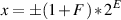 | (8.3) |
where the sign + or - is determined by the value of the sign, F is the fraction (or mantissa) and E is the exponent. The value of F is limited to
 | (8.4) |
Also, we’re going to want to make values of x that are either big or small, therefore the value of E will have to be either positive or negative, respectively.
Keeping in mind that we’re representing our three components using binary numbers, let’s build a simple floating-point system where we have 1 bit for the sign (we don’t need more than this because there are only two possibilities for this value), 2 bits to represent the fraction and 2 bits for the exponent. If we’re going to use this system, then we have a couple of problems to solve.
Firstly, we need to make 0 ≤ F < 1. This is not really a big deal – actually we can use the same system we did for fixed-point to do this. In our system with a 2 bit value for the fraction, we know that we have 4 possible values – in binary, 00, 01, 10 and 11 (or, in decimal, 0, 1, 2, and 3). Let’s call those values F′ So, we’ll just divide those values by 4 to get the value of F . If we had more bits for F′, we’d have to divide by a bigger number to get F . In fact, if we say that we have n bits to represent F′, then we can say that
 | (8.5) |
So, in our 2-bit system, F can equal (in decimal) 0, 0.25, 0.5, or 0.75.
Secondly, we have to represent the exponent, E, using a binary number (in this particular example, with 2 bits) but we want it to be either positive or negative. “That’s easy,” I hear you say, “We’ll just use the two’s complement system.” Sorry... That’s not the way we do it, unfortunately. Let’s call the binary number that’s used to represent the exponent E′. in our 2-bit system, E′ has 4 possible values – in binary, 00, 01, 10 and 11 (or, in decimal, 0, 1, 2, and 3). To convert these to E, we just do a little math again. Let’s say that we have m bits to represent E′, then we say that
 | (8.6) |
So, in our 2-bit system, E can equal (in decimal) -1, 0, 1 or 2.
Now, knowing the possible values for F and E in our system, going back to Equation 8.3, we can find all the possible values for x that we can represent in our binary floating point system. These are all listed in Table 8.2.
| S’ | F’ | E’ | Decimal value |
| 0 | 00 | 00 | 0.500 |
| 0 | 01 | 00 | 0.625 |
| 0 | 10 | 00 | 0.750 |
| 0 | 11 | 00 | 0.875 |
| 0 | 00 | 01 | 1.000 |
| 0 | 01 | 01 | 1.250 |
| 0 | 10 | 01 | 1.500 |
| 0 | 11 | 01 | 1.750 |
| 0 | 00 | 10 | 2.000 |
| 0 | 01 | 10 | 2.500 |
| 0 | 10 | 10 | 3.000 |
| 0 | 11 | 10 | 3.500 |
| 0 | 00 | 11 | 4.000 |
| 0 | 01 | 11 | 5.000 |
| 0 | 10 | 11 | 6.000 |
| 0 | 11 | 11 | 7.000 |
| 1 | 00 | 00 | -0.500 |
| 1 | 01 | 00 | -0.625 |
| 1 | 10 | 00 | -0.750 |
| 1 | 11 | 00 | -0.875 |
| 1 | 00 | 01 | -1.000 |
| 1 | 01 | 01 | -1.250 |
| 1 | 10 | 01 | -1.500 |
| 1 | 11 | 01 | -1.750 |
| 1 | 00 | 10 | -2.000 |
| 1 | 01 | 10 | -2.500 |
| 1 | 10 | 10 | -3.000 |
| 1 | 11 | 10 | -3.500 |
| 1 | 00 | 11 | -4.000 |
| 1 | 01 | 11 | -5.000 |
| 1 | 10 | 11 | -6.000 |
| 1 | 11 | 11 | -7.000 |
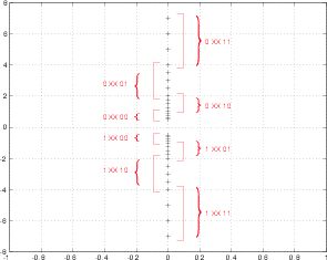
There are a couple of things to notice here about the results listed in Table 8.2 and shown in Figure 8.79. Firstly, notice that we can’t represent the value 0. This might cause us some grief later... Secondly, notice that we do not have equal spacing between the values over the entire range of values. The closer we get to 0, the closer the values are to each other. Thirdly, notice that the change in separation is not constant. We have groups with equal spacing (indicated in Figure 8.79 with the square brackets).
There are a couple of more subtle things to notice in the results of our system. Firstly, look in Table 8.2 at the relationship between the final decimal values and the value of E′. You’ll see that the biggest numbers correspond to the largest value of E′. Consequently, you will see in more technical descriptions of the binary floating point system that the value of the exponent determines the range of the system. More precisely, you’ll see sentences like “the finiteness of [the exponent] is a limitation on [the] range” [Moler, 1996]. This means that the smaller the exponent is, the smaller the range of values in your end result.
Secondly, and less evidently, is the significance of the fraction. Remember that the fraction is scaled to be a value from 0 to less than 1. This means that the more bits we assign to F′, the more divisions of the interval between 0 and 1 that we have. Therefore, the size of the value of F′ in bits determines the precision of our system. More technically, the “finiteness of [the fraction] is a limitation on precision” [Moler, 1996]. This means that the smaller the fraction is, the less precise we can express the value – in other words, the worse the quantization.
“Quantization!” I hear you cry. “Floating point systems shouldn’t have quantization error!” Unfortunately, this is not the case. Floating point systems suffer from quantization error just like fixed point system, however the quantization error is a little weirder. You’ll recall that, in a fixed point system, the quantization error has a maximum value of one-half an LSB. This is true no matter what the value of the signal is, because the entire range is divided equally with equal spacings between quantization values. As we can see in Figure 8.79, in a floating point system, the quantization error is not the same over the entire range. The smaller the value, the smaller the quantization error.
Okay, so there should be one basic question remaining at this point... “How do we express a value of 0 in a binary floating point system?”
FIND OUT THE ANSWER TO THIS QUESTION
Since 1985, there has been an international standard format for floating point binary arithmetic called ANSI/IEEE Standard 754-1985[?]. This document describes how a floating point number should be stored and transmitted. The system we saw above is basically a scaled-down version of this description. If we have 64 bits to represent the binary floating point number, then IEEE 754-1985 states that these bits should be arranged as is shown in Figure 8.80. This is what is called the IEEE double precision format. There are single precision (32 bit) and extended precision (XXX bits) formats as well, but we won’t bother talking about them here.

Given this construction, we can see that E′ has 11 bits and can therefore represent a number from 0 to 2047 (therefore -1022 ≤ E ≤ 1023. F′ can represent a number between 0 and about 4.5036 x 10¹⁵. These two components (with the sign, S′) are assembled to represent a single number x using Equations 8.5, 8.6 and 8.3:
We can calculate the smallest and largest possible values that we can express using this 64-bit system as follows:
The smallest possible value is found when F = 0 and E = -1022. Using Equation 8.3 we find that this value is 2-1022 which is about 2.225*1--308.
The largest possible number is found when F′ is at a maximum and E = 1023. When F′ is at maximum, then F ≈ 1-2.22*10-16. Therefore, using Equation 8.3, we can find that the maximum value is about 1.7977*10308.
NOT YET WRITTEN
NOT YET WRITTEN
MATLAB paper: Floating Points: IEEE Standard Unifies Arithmetic Model: Cleve Moler, Cleve’s Corner, PDF File from The MathWorks (moler:96)
Jamie’s textbook
NOT YET WRITTEN
Back in the days when digital audio was first developed, it was considered that a couple of limits on the audio quality were acceptable. Firstly, it was decided that the sampling rate should be at least high enough to provide the capability of recording and reproducing a 20 kHz signal. This means a sampling rate of at least 40 kHz. Secondly, a dynamic range of around 100 dB was considered to be adequate. Since a word length of 16 bits (a convenient power of 2) gives a dynamic range of about 93 dB after proper dithering, that was decided to be the magic number.
However, as we all know, the business of audio is all about providing more above all else, therefore the resolution of commercially-available digital audio, both in the temporal and level domains, had to be increased. There are some less-cynical arguments for increasing these resolutions.
One argument is that the rather poor (sic) quality of 44.1/16 (kHz and bits respectively) audio is inadequate for any professional recording. This might be supportable were it not for the proliferation of MP3 files throughout the world. Consumption indicates that the general consumer is more and more satisfied with the quality of data-compressed audio which is considerably worse than CD-quality audio. Therefore one might conclude that it makes no sense for manufacturers to be developing systems that have a higher audio quality than a CD.
Another argument is that it is desirable that we return to the old hierarchy where the professionals had access to a much higher quality of recording and reproduction device than the consumers. Back in the old days, we had 1/2-inch 30-ips reel-reel analog tape in the studios and 33-1/3 RPM vinyl LP’s in the consumers’ homes. This meant that the audio quality of the studio equipment was much, much higher than that in the homes, and that we in the studios could get away with murder. You see, if the resolution of your playback system is so bad that you can’t hear the errors caused by the recording, editing and mastering system then the recording, editing and mastering engineers can hear things that the consumer can’t – an excellent situation for quality control. The introduction of digital media to the professional and consumer markets meant that you can could suddenly hear at home exactly what the professionals heard. And, if you spent a little more than they did on a DAC, amplifier and loudspeaker, you could hear things that the pro’s couldn’t... a very bad situation for quality control...
To quote a friend of mine, I stand very firmly on both sides of the fence – I can see that there might be some very good reasons for going to high-resolution digital audio, but I also think that the biggest reason is probably marketing. I’ll try to write this section in an unbiased fashion, but you’d better keep my personal cynicism in mind as you read...
As it became possible, in terms of processing power, storage and transmission bandwidth, people started demanding more from their digital audio. As we’ve seen, there are two simple ways to describe the resolution (if not the quality level) of digital audio – the sampling rate and the word length. In order to make digital audio systems that were better (or at least appeared on paper to be better) these two numbers had to get bigger. As ADC and DAC design improved, it became easier to increase the word length to 24 bits. Twenty-four was chosen to be a good number since the AES/EBU protocol was designed to support a 24-bit word length and since 141 dB was decided to be an adequate signal to noise ratio. In order to increase the sampling rate, we just started multiplying by 2, starting with the two standard sampling rates. We now have 88.1, 96, 176.4 and 192 kHz, among others.
When the folks that came up with DVD-Audio sat down to decide on the specifications for the media, they made it possible for the disc to support 24 bits and the various sampling rates listed above. (However, people were using higher sampling rates before DVD-Audio came around – it was just harder to get it into people’s homes.) The term “high resolution” audio was already being thrown around by the time of the introduction of DVD-Audio to describe sampling rates higher than 44.1 or 48 kHz and word lengths longer than 16 bits.
One of the problems with DVD-Audio is a marketing problem – it is not backwards compatible with the CD format. Although a DVD-Audio player can play a CD, a CD player cannot play a DVD-Audio. So, the folks at Sony and Philips saw a marketing niche. Instead of supporting the DVD-Audio format, they decided to come up with a competing format called Super Audio Compact Disc or SACD. As is described below, this format is based on Delta-Sigma conversion at a very high sampling rate of approximately 2.83 MHz. Through some smart usage of the two layers on the disc, the format was designed with a CD-compatible layer so that a hybrid disc could be manufactured – one that could play on an old-fashioned CD player.
We’ll look at the specifics of the formats in later sections.
It didn’t take long for the fascination with compact discs and Digital Audio Tapes to wear off and for people to want more. There were many complaints in the early 80’s about all of the problems with digital audio. Words like “harsh” and “brittle” were being thrown around a lot. There are a couple of reasonable explanations for this assessment. The early ones suggested that digital audio inherently produced symmetrical distortion (producing artifacts in odd harmonics) whereas analog produced asymmetrical distortion (therefore producing even harmonics). People say that even harmonic distortion sounds “better” than odd harmonic distortion, therefore analog is better than digital. This argument may or may not necessarily be the case, but it gave people something to talk about. (In fact, this argument is a throwback to the reasons for buying tubes (or valves, depending on which side of the Atlantic Ocean you’re from) versus transistors.)
Some other explanations hinged on the general idea of distortion. Namely, that analog reproduction systems, particularly vinyl, distorted the recorded signal. Things like wow and flutter or analog tape compression were commonplace in the days of analog recording. When CD’s hit the scene, these things disappeared (except maybe for tape compression from the original analog recordings...). It is possible that people developed a preference for such types of distortion on their audio, so when the distortion was removed, they didn’t like it as much.
Another reason that might be attributable to the problems in early digital audio was the quality of the converters. Twenty years ago, it wasn’t so easy to build a decent analog-to-digital converter with an accuracy equivalent to 16 bits. In fact, if you do a measurement of some of the DAT machines from the early 80’s you’ll find that the signal-to-noise ratio was equivalent to about 12 or 13 bits. On top of this, people really didn’t know how to implement dither properly, so the noise floor was primarily distortion. This automatically puts you in the land of harsh and brittle...
Yet another possible explanation for the problems in early digital audio lies in the anti-aliasing filters used in the DAC’s. Nowadays, we use analog filters with gentle slopes feeding oversampled DAC’s followed by digital filters before the digital signal is downsampled to the required resolution for storage or transmission. Early converters were slightly different because we didn’t have enough computational power to run either the oversampled DAC or the digital filters, so the filters were implemented in analog circuitry. These analog filters had extremely high slopes, and therefore big phase shifts around the cutoff frequency, resulting in ringing. This ringing is still audible in the recordings that were made in that era.
Today, many people still aren’t happy with the “standard” sampling rates of 44.1 and 48 kHz, nor are they satisfied with a 16-bit word length, although to the best of my knowledge, there haven’t been any trustworthy listening tests whose results have conclusively proven that going to higher resolutions produces audible results.
There are a number of suggestions that people have put forward regarding why higher resolutions are necessary – or at least desirable in digital audio. I’ve listed a couple of these reasons below with some explanations as to why they may or may not be worth listening to.
This is one of the first arguments you’ll hear for higher sampling rates. Many people claim that there are multiple benefits to increasing the upper cutoff frequency of our recording systems, requiring higher sampling rates. Remember that the original sampling rates were chosen to be adequate to record audio content up to and including 20 kHz. This number is ubiquitous in our literature regarding the upper limits of human hearing – every student that learns anything about psychoacoustics starts off on day one learning that audible sound ranges from 20 Hz to 20 kHz, as if we had two brick wall filters in our ears.
One group makes its claims on frequency response measurements of the outputs of instruments[Boyk, 1992]. The logic is that since the instruments (such as a trumpet with a harmon mute as a notable example) produce relatively high-level content above 20 kHz, our recording systems must capture this content. Therefore, we need higher sampling rates. One can show that humans are unable to hear sine tones of a reasonable level with frequencies above 20 kHz. However, it is possible that complex tones with harmonic content above 20 kHz produce resultant tones that may or may not be audible. It could be argued that these resultant tones are not audible with real sources in real life, but would be audible but undesirable in loudspeakers resulting from intermodulation distortion (described in Section ??). (If you would like to test yourself in this area, do an experiment where you’re asked to tell the difference between a square wave and a sine wave, both with a fundamental frequency of 7 kHz. If you can hear the difference between these two (make sure that they’re the same level!) then these people have a point. You see, the only difference between a sine wave a square wave is the energy in the odd harmonics above the fundamental in the square wave. Since the first odd harmonic above the fundamental is 3 times the fundamental, then all of the differences between the two tones at 7 kHz will be content at 21 kHz and higher. In cased you’re interested, I tried this experiment and none of my subjects (including me) were able to tell the difference with any reliability.)
Another group relies on the idea that our common understanding of human limits of hearing is incorrect. For many years, many people have argued that our hearing does not stop at 20 kHz, regardless of what the tests and textbooks tell us. These folks say that we are actually able to perceive spectral content above 20 kHz in one way or another. When it proved to be impossible to get people to identify such things in standard listening tests (i.e. can you hear the difference between two sounds, one band-limited and one not) people resorted to looking at EKG’s to see if high-frequency content changed Alpha-waves[Yamamoto et al., 1994][Yoshikawa et al., 1995][Yoshikawa et al., 1997].
Once upon a time, there was a voice of sanity in the midst of the noise. Listserves and newgroups on Usenet would be filled with people spouting opinions on why bigger was better when it came to numbers describing digital audio. All sorts of strange ideas were (are) put forward by people who don’t know the quote by George Eliot – “Blessed is the man who, having nothing to say, abstains from giving in words evidence to that fact” or a similar piece of advice from Abraham Lincoln – “Better to be thought a fool than to open your mouth and remove all doubt.” The lonely voice of sanity belonged to a man named Julian Dunn. Mr. Dunn wrote a paper that suggested that there was a very good reason why higher sampling rate may result in better sounding audio even if you can’t hear above 20 kHz[Dunn, 1998]. He showed that the antialiasing filters used within ADC’s do not have a flat frequency response in their passband. And, not only was their frequency response not flat, but they typically have a periodic ripple in the frequency domain. Of course, there’s a catch – the ripple that we’re talking about is on the order of 0.1 dB peak-to-peak, so we’re not talking about a big problem here...
The interesting thing is that this frequency response irregularity can be reduced by increasing your sampling rate and reducing the slope of the antialiasing filters. Therefore, it’s possible that higher sampling rates sound better because of reduced artifacts in the audio band of 20 Hz – 20 kHz caused by the filters.
Dunn also noted that, if you’re smart, you can design your reconstruction filter in your DAC to have the same ripple with the opposite phase (in the frequency domain), thus canceling the effects of both filters and producing a perfectly flat response of the total system. Of course, this would mean that all manufacturers of ADC’s and DAC’s would have to use the same filters and that would, in turn mean that no converter would sound better than another which would screw up the pricing structure of that market... So most people that make converters (especially expensive ones) probably think that this is a bad idea.
You can download a copy of this paper from the web at www.nanophon.com.
When students are learning PCM digital audio for the very first time, an analogy is made to film. Film takes 24 snapshots per second of the action and plays them back at the same speed to resemble motion. Similarly, PCM digital audio takes a much larger number of “snapshots” of the voltage level of the signal each second and plays them back later in the same order to reconstruct the signal.
This is a pretty good analogy (which is why I used it back in Section 8.1). However, it causes a misconception later. If we stick with thinking about film for a moment, we have a limited temporal resolution. For example, if an event happens, lasting for a very short period of time and occurring between two frames of the film, then the event will never be recorded on the film. Let’s say that you’re making a movie of a wedding and somebody snaps a photograph with a flash. Let’s also pretend that the flash lasts only for 1/60th of a second (faster than your 1/24th of a second frame rate) and that flash happens between frames of your movie. When you play back the movie, you’ll never see the flash because it happened at a moment in time that your film didn’t record.
There are a large number of people in the audio world who are under the misconception that this also holds true in digital audio. The belief is that an event that happens between two samples will not be recorded. Consequently, things like precise time of arrival at a microphones or multiple reflections arriving at very closely spaced intervals will not be recorded because their arrival doesn’t correspond to a sample time. Or, another belief is that the time of arrival is quantized in time to the nearest sample, so differences in times of arrival of a wavefront at two microphones will be slightly altered, rounding off to the nearest sample.
I want to express this as explicitly as possible... People who think this are just plain wrong.
Let’s pretend for a minute that recording sound in the digital domain actually caused temporal quantization and think about some of the consequences...
So, as you can see, since none of these three things happen, then temporal resolution in the digital domain must be infinite. So, please do not listen to people when they tell you that higher sampling rates are better because it gives a better representation of the time information in the signal.
The sampling period has no relationship whatsoever with the ability of a digital recording system (either PCM or Delta-Sigma) to resolve the time of a signal. This is because the signal is filtered by the anti-aliasing filters. A discrete time audio system (i.e. digital) has an infinite resolution in the temporal domain if the signal is properly band-limited.
| Sampling Rate | Sampling Period | Temporal Resolution |
| 44.1 kHz | 22.7 μsec | |
| 48 kHz | 20.8 μsec | |
| 88.2 kHz | 11.3 μsec | |
| 96 kHz | 10.4 μsec |  sec sec |
| 192 kHz | 5.3 μsec | |
| 384 kHz | 2.6 μsec | |
| 2.83 MHz | 0.35 μsec | |
Do not take everything I’ve said in this chapter as the definitive reference on the subject of high-resolution audio. Go read the papers by Julian Dunn and Malcom Hawkesford and a bunch of other people before you make up your mind on whether it’s worth the disc space to do recordings at 96 kHz or higher. However, don’t base your decisions on one demo from a marketing rep of a company who’s trying to sell you a product. And don’t get sucked in by the simple marketing ploy that “more” and “better” are equivalent terms.
Malcolm Hawkesford
Julian Dunn
NOT YET WRITTEN
Back in 1983, a new format for playing audio was introduced to the consumer market that represented a radical shift in the relationship between professional and consumer quality. The advertisements read “Perfect sound... forever...” Of course, we now know that most early digital recordings were far from “perfect” (whatever that word entails) and that compact discs don’t last forever.
The compact disc or “CD” format was developed as a cooperative effort between Sony and Philips. It was intended from the very beginning to be a replacement format for vinyl LP’s – a position that it eventually secured in all but two markets (being the DJ and the hard-core audiophile markets).
In initially developing the CD format, Sony and Phillips had to make many decisions regarding the standard. Three of the most basic requirements that they set were the sampling rate, the bit depth and the total maximum playing time.
Nowadays, when we want to do a digital recording, we either show up with a DAT machine, or a laptop with an audio input, writing data straight to our hard drives. Back in the 1980’s however, DAT hadn’t been invented yet, and hard discs just weren’t fast enough to cope with the data rate required by digital audio. The only widely-available format that could be used to record the necessary bandwidth was a video recorder. Consequently, machines were built that took a two-channel audio input, converted that to digital and sent a video output designed to be recorded on either a Beta tape if you didn’t have a lot of money (yes... Beta... if you’re too young, you may not have even heard of this format. If you’re at least as old as me, you probably have some old recordings still lying around on Beta tapes...) or U-Matic if you did. (U-Matic is an old analog professional-format video tape that uses 3/4” tape.)The process of converting from digital audio to video was actually pretty simple, a 1 was a white spot and a 0 was a black spot. So, if you looked at your digital audio recording on a television, you’d see a bunch of black and white strips, looking mostly like noise (or snow as it’s usually called when you see noise on a TV).
Since the recording format (video tape) was already on the market, the conversion process was, in part, locked to that format. In addition, the manufacturers had to ensure that tapes could be shipped across the Atlantic Ocean and still be useable. This means that the sampling rate had to be derived from, among other things, the frame rates of NTSC and PAL video.
To begin with, it was decided that the minimum sampling rate was 40 kHz to allow for a 20 kHz minimum Nyquist frequency. Remember that the audio samples were stored as black and white stripes in the video signal, so a number above 40 kHz had to be found that fit both formats nicely. NTSC video has 525 lines per frame (of which 490 are usable lines for recording signals) at a frame rate of 29.97 Hz. This can be further divided into 245 usable lines per field (there are 2 fields per frame) at a field rate of 59.95 Hz. If we put 3 audio samples on each line of video, then we arrive at the following equation [Watkinson, 1988]:
59.94 Hz * 245 lines per field * 3 samples per line = 44.0559 Hz
PAL is slightly different. Each frame has 625 lines (with 588 usable lines) at 25 Hz. This corresponds to 294 usable lines per field at a field rate of 50 Hz. Again, with 3 audio samples per line of video, we have the equation [Watkinson, 1988]:
50.00 * 294 lines per field * 3 samples per line = 44.1000 Hz
These two resulting sampling rates were deemed to be close enough (only a 0.1% difference in sampling rate) to be compatible (this difference in sampling rate corresponds to a pitch shift of about 0.0175 of a semitone).
This is perfect, but we’re forgetting one small thing... most people record in stereo. Therefore, the EIAJ format was developed from these equations, resulting in 6 samples per video line (3 for each channel).
There is one odd addition to the story. Technically speaking, the compact disc format really had no ties with video (back in 1983, you couldn’t play video off a CD yet) but the equipment that was used for recording and mastering was video-based. Interestingly, NTSC professional video gear (the U-Matic format) can run at frame rate of 30 fps, and is not locked to the 29.97 of your television at home. Consequently, if you re-do the math with this frame rate, you’ll find that the resulting sampling rate is exactly 44.1 kHz. Therefore, to ensure maximum compatibility and still keep a technically achievable sampling rate, 44.1 kHz was chosen to be the standard.
The next question was that of word length. How many bits are enough to adequately reproduce an audio signal? And, possibly more importantly, what is technically feasible to implement, both in terms of storing the data as well as converting it from and back to the analog domain. We have already seen that there is a direct connection between the number of bits used to describe the signal level and the signal-to-noise ratio incurred in the conversion process.
NOT YET WRITTEN
NOT YET WRITTEN
A compact disc is a disc make primarily of a polycarbonate plastic made by Bayer and called Makrolon [Watkinson, 1988]. This is supplied to the CD manufacturer as small beads shipped in large bags. The disc has a total outer diameter of 120 mm with a 15 mm hole, and the thickness is 1.2 mm.
The data on the disc plays from the inside to the outside and has a constant bit rate. As a result, as the laser tracks closer and closer to the edge of the disc, the rotational speed must be reduced to ensure that the disc-to-laser speed remains constant at between 1.2 and 1.4 m/s [Watkinson, 1988]. At the very start of the CD, the disc spins at about 230 rpm and at the very end of a long disc, it’s spinning at about 100 rpm. On a full CD, the total length of the spiral path read by the laser is about 5.7 km [Watkinson, 1988].
ADD MORE HERE ABOUT PITS AND LANDS, OR BUMPS...
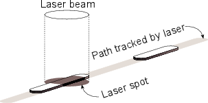
The wavelength λ of the laser light is 0.5 μm. The bump height is 0.13 μm,
corresponding to approximately  for the laser. As a result, when the laser spot is hitting
a bump on the disc, the reflections from both the bump and the adjacent lands (remember
that the laser spot is wider than the bump) results in destructive interference and therefore
cancellation of the reflection. Therefore, seen from the point of view of the pickup, there
is no reflection from a bump.
for the laser. As a result, when the laser spot is hitting
a bump on the disc, the reflections from both the bump and the adjacent lands (remember
that the laser spot is wider than the bump) results in destructive interference and therefore
cancellation of the reflection. Therefore, seen from the point of view of the pickup, there
is no reflection from a bump.
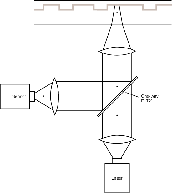
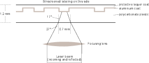
There is a small problem in this system of representing the audio data with bumps on the CD. Let’s think about a worst-case situation where, for some reason, the audio data is nothing but a string of alternating 1’s and 0’s. If we were representing each 0 with a bump and each 1 with a not-bump, then, even if we didn’t have additional information to put on the disc (and we do...), we’d be looking at 1,411,200 bump-to-not-bump transitions per second or a frequency of about 1.4 MHz (44.1 kHz x 16 bits per sample x 2 channels). Unfortunately, it’s not possible for the optical system used in CD’s to respond that quickly – there’s a cutoff frequency for the data rate imposed by a couple of things (such as “the numerical aperture of the optics and the track velocity” [Watkinson, 1988]). In addition, we want to keep our data rate below this cutoff to gain some immunity from problems caused by “disc warps and focus errors” [Watkinson, 1988].
So, one goal is to somehow magically reduce the data rate from the disc as low as possible. However, this will cause us another problem. The data rate of the bits going to the DAC is still just over 705 kHz (44.1 kHz x 16 bits per sample). This clock rate has to be locked to, or derived from the data coming off the disc itself, which we have already established, can’t go that fast... If the data coming off the disc is too slow, then we’ll have problems locking our slow data rate from the disc with the fast data rate of information getting to the DAC. If this doesn’t make sense at the moment, stick with me for a little while and things might clear up.
So, we know that we need to reduce the amount of data written to (and read from) the disc without losing any audio information. However, we also know that we can’t reduce the data rate too much, or we’ll introduce jitter at best and locking problems at worst. The solution to this problem lies in a little piece of magic called eight to fourteen modulation or EFM.
To begin with, eight to fourteen modulation is based on a lookup table. A small portion of this table is shown in Table 8.4.
We being by taking each 16-bit sample that we want to put on the disc and slice it into two 8-bit bytes. We then go to the table and look up the 8-bit value in the middle column of Table 8.4. The right-hand column shows a different number containing 14 bits, so we write this down.
For example, let’s say that we want to put the number 01101001 on the disc. We go to the table, look up that number and we get the corresponding number 10000001000010.
| Data value | Data bits | Channel bits |
| (decimal) | (binary) | (binary) |
| 101 | 01100101 | 00000000100010 |
| 102 | 01100110 | 01000000100100 |
| 103 | 01100111 | 00100100100010 |
| 104 | 01101000 | 01001001000010 |
| 105 | 01101001 | 10000001000010 |
| 106 | 01101010 | 10010001000010 |
| 107 | 01101011 | 10001001000010 |
| 108 | 01101100 | 01000001000010 |
| 109 | 01101101 | 00000001000010 |
| 110 | 01101110 | 00010001000010 |
Okay, so right about now, you should be saying “I thought that we wanted to reduce the amount of data... not increase it from 8 up to 14 bits...” We’re getting there.
What we now do is to take our 14-bit word 10000001000010 and draw an irregular pulse wave where we have a transition (from high to low or low to high) for every “1” in the word. This is illustrated in Figure 8.84. Compare the examples in this figure with the corresponding 14-bit values in Table 8.4.

Okay, we’re not out of the woods yet. We can still have a problem. What if the 14-bit word has a string of 1’s in it? Aren’t we still stuck with the original problem, only worse? Well, yes. But, the clever people that came up with this idea were very careful about choosing their 14-bit representative words. They made sure that there are no 14-bit values with 1’s separated be less than two 0’s. Huh? For example, none of the 14-bit words in the lookup table contain the codes 11 or 101 anywhere. Take a look at the small example in Table 8.4. You won’t find any 1’s that close together - minimum separation of two 0’s at any time. In real textbooks they talk about a minimum period between transitions of 3T where T is the period of 1 bit in the 14-bit word. (This period T is 231.4 ns, corresponding to a data rate of 4.3218 MHz [Watkinson, 1988] – but remember, that’s the data rate of the 14-bit word, not the signal stamped on the disc.) This guarantees that the transition rate on the disc cannot exceed 720 kHz, which is high, but acceptable.
So, that looks after the highest frequency, but what about the lowest possible frequency of bump transitions? This is looked after by setting a maximum period between transitions of 11T , therefore there are no 14-bit words with more than ten 0’s between 1’s. This sets our minimum transition frequency to 196 kHz which is low, but acceptable.
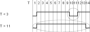
Let’s talk a little more about why we have this low-frequency limitation on the data rate. Remember that when we talk about a “period between transitions of 11T ” we’re directly talking about the length of the bump (or not-bump) on the disc surface. We’re already seen that the rotational speed of the disc is constantly changing as the laser gets further and further away from the centre. This speed change is done in order to keep the data rate constant – the physical length of a bump of 9T at the beginning of the disc is the same as that of a bump of 9T at the end of the disc. The problem is, if you’re the sensor responsible for converting bump length into a number, you really need to know how to measure the bump length. The longer the bump, the more difficult it is to determine the length, because it’s a longer time since the last transition.
To get an idea of what this would be like, stand next to a train track and watch a slowing train as it goes by. Count the cars, and get used to the speed at which they’re going by, and how much they’re slowing down. Then close your eyes and keep counting the cars. If you had to count for 3 cars, you’d probably be pretty close to being right in synch with the train. If you had to count 9 cars, you’d probably be wrong, or at least losing synchronization with the train. This is exactly the same problem that the laser sensor has in estimating pit lengths. The longer the pit, the more likely the error, so we keep a maximum of 11T to minimize the likelihood of errors.
One problem that digital audio introduces is the issue of bandwidth and disk space. If you want to record something to tape and you know that it’s going to last about an hour and a half, then you go and buy a two-hour tape. If you’re recording to a hard drive, and you have 700 MB available, how much time is that?
In order to calculate this, you’ll need to consider the bandwidth of the signal you’re going to send. Consider that, for each channel of audio, you’re going to some number of samples, depending on the sampling rate, and each of those samples is going to have some number of bits, depending on the word length.
Let’s use the example of CD to make a calculation. CD uses a sampling rate of 44.1 kHz (44100 samples per second) and 16-bit word lengths for two channels of audio. Therefore, each second, in each of two channels, 44100, 16-bit numbers come through the system. So:
2 channels
* 44100 samples per second
* 16 bits per sample
= 1,411,200 bits per second
What does this mean in terms of disc space? In order to calculate this, we just have to convert the number of bits into the typical storage unit for computers – a byte (eight bits).
1,411,200 bits per second
/ 8 bits per byte
= 176,400 bytes per second
divide that by 1024 (bytes per kilobyte) and we get the value in kilobytes per second, resulting in a value of 172.27 kB per second.
From there we can calculate into what are probably more meaningful terms:
172.27 kB per second
* 60 seconds per minute
= 10,335.94 kilobyte per minute
/ 1024 kilobyte per megabyte
= 10.1 MB per minute.
So, when you’re storing uncompressed, CD-quality audio on your hard drive, it’s occupying a little more than 10 MB per minute of space, so 700 MB of free space is about 70 minutes of music.