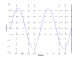
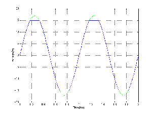
Figure 10.1: A 1 kHz sine wave without distortion worth talking about.
Thanks to Claudia Haase and Thomas Lischker at RTW Radio–Technische (www.rtw.de) for their kind permission to use graphics from their product line for this section.
When you sit down to do a recording – any recording, you have two basic objectives:
1) make the recording sound nice aesthetically
2) make sure that the technical quality of the recording is high.
Different people and record labels will place their priorities differently (I’m not going to mention any names here, but you know who you are...)
One of the easiest ways to guarantee a high technical quality is to pay particular attention to your gain and levels at various points in the recording chain. This sentence is true not only for the signal as it passes out and into various pieces of equipment (i.e. from a mixer output to a tape recorder input), but also as it passes through various stages within one piece of equipment (in particular, the signal level as it passes through a mixer). The question is: “what’s the best level for the signal at this point in the recording chain?”
There are two beasts hidden in your equipment that you are constantly trying to avoid and conceal as you do your recording. On a very general level, these are noise and distortion.
Noise can be generally defined as any audio in the signal that you don’t want there. If we restrict ourselves to electrical noise in recording equipment, then we’re basically talking about hiss and hum. The reasons for this noise and how to reduce it are discussed in a different chapter, however, the one inescapable fact is that noise cannot be avoided. It can be reduced, but never eliminated. If you turn on any piece of audio equipment, or any component within any piece of equipment, you get noise. Normally, because the noise stays at a relatively constant level over a long period of time and because we don’t bother recording signals lower in level than the noise, we call it a noise floor.
How do we deal with this problem? The answer is actually quite simple: we turn up the level of the signal so that it’s much louder than the noise. We then rely on psychoacoustic masking (and, if we’re really lucky, the threshold of hearing) to cover up the fact that the noise is there. We don’t eliminate the noise, we just hide it – and the louder we can make the signal, the better it’s hidden. This works great, except that we can’t keep increasing the level of the signal because at some point, we start to distort it.
If the recording system was absolutely perfect, then the signal at its output would be identical to the signal at the input of the microphone. Of course, this isn’t possible. Even if we ignore the noise floor, the signals at the two ends of the system are not identical – the system itself modifies or distorts the signal a little bit. The less the modification, the lower the distortion of the signal and the better it sounds.
Keep in mind that the term “distortion” is extremely general – different pieces of equipment and different systems will have different detrimental effects on different signals. There are different ways of measuring this, but we typically look at the amount of distortion in percent. This is a measurement of how much extra power is included in the signal that shouldn’t be there. The higher the percentage, the more distortion and the worse the signal. (See the chapter on distortion measurements in the Electroacoustic Measurements section.)
There are two basic causes of distortion in any given piece of equipment. The first is the normal day–to–day error of the equipment in transmitting or recording the signal. No piece of gear is perfect, and the error that’s added to the signal at the output is basically always there. The second, however, is a distortion of the signal caused by the fact that the level of the signal is too high. The output of every piece of equipment has a maximum voltage level that cannot be exceeded. If the level of the signal is set so high that it should be greater than the maximum output, then the signal is clipped at the maximum voltage as is shown in Figure 10.2.
For our purposes at this point in the discussion, I’m going to over–simplify the situation a bit and jump to a hasty conclusion. Distortion can be classified as a process that generates unwanted signals that are added to our program material. In fact, this is exactly what happens – but the unwanted signals are almost always harmonically related to the signal whereas your run–of–the–mill noise floor is completely unrelated harmonically to the signal. Therefore, we can group distortion with noise under the heading “stuff we don’t want to hear” and look at the level of that material as compared to the level of the program material we’re recording – in other words the “stuff we do want to hear.” This is a small part of the reason that you’ll usually see a measurement called “THD+N” which stands for “Total Harmonic Distortion plus Noise” – the stuff we don’t want to hear.
So, we need to make the signal loud enough to mask the noise floor, but quiet enough so that it doesn’t distort, thus maximizing the level of the signal compared to the level of the distortion and noise components. How do we do that? And, more importantly, how do we keep the signal at an optimal level so that we have the highest level of technical quality? In order to answer this question, we have to know the exact behaviour of the particular piece of gear that we’re using – but we can make some general rules that apply for groups of gear. These three groups are 1) digital gear, 2) analog electronics and 3) analog tape.
As we’ve seen in previous chapters, digital gear has relatively easily defined extremes for the audio signal. The noise floor is set by the level of the dither, typically with a level of one half of an LSB. The signal to noise ratio of the digital system is dependent on the number of bits that are used for the signal – increasing by 6.02 dB per bit used. Since the level of the dither is typically half a bit in amplitude, we subtract 3 dB from our signal to noise ratio calculated from the number of bits. For example, if we are recording a sine wave that is using 12 of the 16 bits on a CD and we make the usual assumptions about the dither level, then the signal to noise ratio for that particular sine wave is:
(12 bits * 6 dB per bit) – 3 dB
= 69 dB
Therefore, in the above example, we can say that the noise floor is 69 dB below the signal level. The more bits we use for the signal (and therefore the higher its peak level) the greater the signal to noise ratio and therefore the better the technical quality of the recording. (Do not confuse the signal to noise ratio with the dynamic range of the system. The former is the ratio between the signal and the noise floor. The latter is the ratio between the maximum possible signal and the noise floor – as we’ll see, this raises the question of how to define the maximum possible level...)
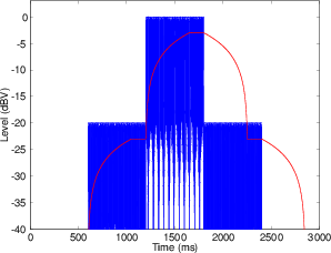
We also know from previous chapters that digital systems have a very unforgiving maximum level. If you have a 16 bit system, then the peak level of the signal can only go to the maximum level of the system defined by those 16 bits. There is some debate regarding what you can get away with when you hit that wall – some people say that 2 consecutive samples at the maximum level constitutes a clipped signal. Others are more lenient and accept one or two more consecutively clipped samples. Ignoring this debate, we can all agree that, once the peak of a sine wave has reached the maximum allowable level in a digital system, any increase in level results in a very rapid increase in distortion. If the system is perfectly aligned, then the sine wave starts to approach a square wave very quickly (ignoring a very small asymmetry caused by the fact that there is one extra LSB for the negative–going portion of the wave than there is for the positive side in a PCM system). See Figure 10.2 to see a sample input and output waveform. The “consecutively clipped samples” that we’re talking about is a measurement of how long the flattened part of the waveform stays flat.
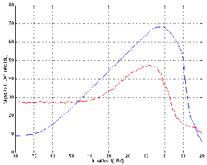
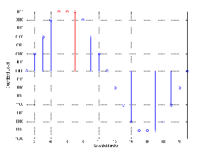
If we were to draw a graph of this behaviour, we would result in the plot shown in Figure 10.3. Notice that we’re looking at the Signal to THD+N ratio vs. the level of the signal.
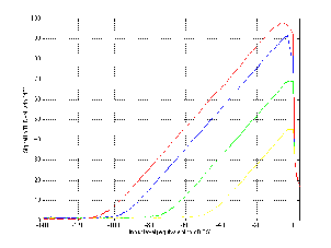
The interesting thing about this graph is that it’s essentially a graph of the peak signal level vs. audio quality (at least technically speaking... we’re not talking about the quality of your mix or the ability of your performers...). We can consider that the X–axis is the peak signal level in dB FS and the Y–axis is a measurement of the quality of the signal. Consequently, we can see that the closer we can get the peak of the signal to 0 dB FS the better the quality, but if we try to increase the level beyond that, we get very bad very quickly.
Therefore, the general moral of the story here is that you should set your levels so that the highest peak in the signal for the recording will hit as close to 0 dB FS as you can get without going over it. In fact, there are some problems with this – you may actually wind up with a signal that’s greater than 0 dB FS by recording a signal that’s less than 0 dB FS in some situations... but we’ll look at that later... this is still the introduction.
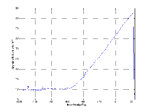
Analog electronics (well, operational amplifiers really... but pretty well everything these days is built with op amps, so we’ll stick with the generalized assumption for now...) have pretty much the same distortion characteristics as digital, but with a lower noise floor (unless you have a very high resolution digital system or a really crappy analog system). As can be seen in Figure 10.4, the general curve for an analog microphone preamplifier, mixing console, or equalizer (note that we’re not talking about dynamic range controllers like compressors, limiters, expanders and gates) looks the same as the curve for digital gear shown in Figure 10.3. If you’ve got a decent piece of analog gear (even something as cheap as a Mackie mixer these days) then you should be able to hit a maximum signal to noise ratio of about 125 dB or so when the signal is at some maximum level where the peak level is bordering on the clipping level (somewhere around +/- 13.5 V or +/- 16.5 V, depending on the power supply rails and the op amps used). Any signal that goes beyond that peak level causes the op amps to start clipping and the distortion goes up rapidly (and bringing the quality level down quickly).
So, the moral of the story here is the same as in the digital world. As a general rule, it’s good for analog electronics to keep your signal as high as possible without hitting the maximum output level and therefore clipping your signal.
One minor problem in the analog electronics world is knowing exactly what level causes your gear to distort. Typically, you can’t trust your meters as we’ll see later, so you’ll either have to come up with an alternate metering method (either using an oscilloscope, an external meter, or one of your other pieces of gear as the meter) or just keep your levels slightly lower than optimal to ensure that you don’t hit any brick walls.
One nice trick that you can use is in the specific case where you’re coming from an analog microphone preamplifier or analog console into a digital converter (depending on its meters). In this case, you can pre–set the gain at the input stage of the mic pre such that the level that causes the output stage of the mixer to clip is also the level that causes the input stage of the ADC to clip. In this case, the meters on your converter can be used instead of the output meters on your microphone preamplifier or console. If all the gear clips at the same level and your stay just below that level at the recording’s peak, then you’ve done a good job. The nice thing about this setup is that you only need to worry about one meter for the whole system.
Analog tape is a different kettle of fish. The noise floor in this case is the same as in the analog and digital worlds. There is some absolute noise floor that is inherent on the tape (the reasons for which are discussed in the chapter on analog tape, oddly enough...) but the distortion characteristics are different.
When the signal level recorded on an analog tape is gradually increased from a low level, we see an increase in the signal to noise ratio because the noise floor stays put and the signal comes up above it. At the same time however, the level of distortion gradually increases. This is substantially different from the situation with digital signals or op amps because the clipping isn’t immediate – it’s a far more gradual process as can be seen in Figure 10.5.
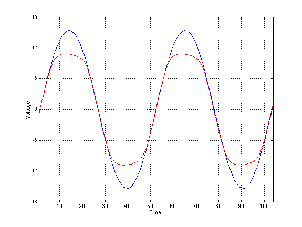
The result of this softer, more gradual clipping of the waveform is twofold. Firstly, as was mentioned above, the increase in distortion is more gradual as the level is increase. In addition, because the change in the slope of the waveform is less abrupt, there are fewer very high frequency components resulting from the distortion. Consequently, there are a large number of people who actually use this distortion as an integral part of their processing. This tape compression as it is commonly known, is most frequently used for tracking drums.
Assuming that we are trying to maintain the highest possible technical quality and assuming that this does not include tape compression, then we are trying to keep the signal level at the high point on the graph in Figure 5. This level of 0 dB VU is a so–called nominal level at which it has been decided (by the tape recorder manufacturer, the analog tape supplier and the technician that works in your studio) that the signal quality is best. Your goal in this case is to keep the average level of the signal for the recording hovering around the 0 dB VU mark. You may go above or below this on peaks and dips – but most of the time, the signal will be at an optimal level.
Notice that there are two fundamentally different ways of thinking presented above. In the case of digital gear or analog electronics, you’re determining your recording level based on the absolute maximum peak for the entire recording. So, if you’re recording an entire symphony, you find out what the loudest part will be and make that point in the recording as close to maximum as possible. Look after the peak and the rest will look after itself. In contrast, in the case of analog tape, we’re not thinking of the peak of the signal, we’re concentrating on the average level of the signal – the peaks will look after themselves.
So, now that we’ve got a very basic idea of the objective, how do we make sure that the levels in our recording system are optimized? We use the meters on the gear to give us a visual indication of the levels. The only problem with this statement is that it assumes that the meter is either telling you what you want to know, or that you know how to read the meter. This isn’t necessarily as dumb as it sounds.
A discussion of meters can be divided into two subtopics. The first is the issue of scale – what actual signal level corresponds to what indication on the meter. The second is the issue of ballistics – how the meter responds in time to changes in level.
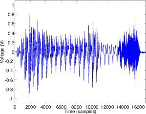
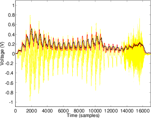
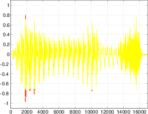
Before we begin, we’ll take a quick review of the difference between the peak and the RMS value of a signal. Figure 10.7 shows a portion of a recorded sound wave. In fact, it’s an excerpt of a recording of male speech.
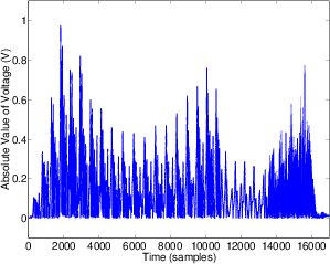
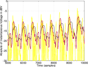
One simple measurement of the signal level is to continuously look at its absolute value. This is simply done by taking the absolute value of the signal shown in Figure 10.8.
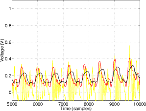
A second, more complex method is to use the running RMS of the signal. As we’ve already discussed, the relationship between the RMS and the instantaneous voltage is dependent on the time constant of the RMS detection circuit. Notice in Figure 10.9 that not only do the highest levels in the RMS signals differ (the shorter the time constant, the higher the level) but their attack and decay slopes differ as well.
A level meter tells you the level of the signal – either the peak or the RMS value of the level depending on the meter – on a relative scale. We’ll look at these one at a time, and deal with the respective scale and ballistics for each.
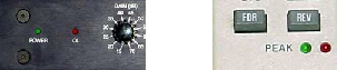
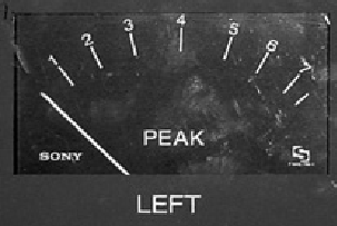
If you look at a microphone preamplifier or the input module of a mixing console, you’ll probably see a red LED. This peak light is designed to light up as a warning signal when the peak level (the instantaneous voltage – or more likely the absolute value of the instantaneous voltage) approaches the voltage where the components inside the equipment will start to clip. More often than not, this level is approximately 3 dB below the clipping level. Therefore, if the device clips at +/– 16.5 V then the peak light will come on if the signal hits 11.6673 V or –11.6673 V (3 dB less than 16.5 V or 16.5 V / sqrt(2)). Remember that the level at which the peak indicator lights is dependent on the clip level of the device in question – unlike many other meters, it does not indicate an absolute signal strength. So, without knowing the exact characterstics of the equipment, we cannot know what the exact level of the signal is when the LED lights. Of course, the moral of that issue is “know your equipment.”
For example, take a look at Figure 10.13. Let’s assume that the signal is passing through a piece of equipment that clips at a maximum voltage of 10 V. The peak indicator will more than likely light up when the signal is 3 dB below this level. Therefore any signal greater than 7.07 V or less than –7.07 V will cause the LED to light up.
Note that a peak indicator is an instantaneous measurement. If all is working properly, then any signal of any duration (no matter how short) will cause the indicator to light if the signal strength is high enough.
Also note that the peak indicator lights when the signal level is slightly lower than the level where clipping starts, so just because the light lights doesn’t mean that you’ve clipped your signal... but you’re really close.
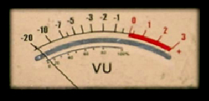
The Volume Unit Meter (better known as a VU Meter) shows what is theoretically an RMS level reading of the signal passing through it. Its display is calibrated in decibels that range from –20 dB VU up to +3 dB VU (the range of 0 dB VU to +3 dB VU are marked in red). Because the VU meter was used primarily for recording to analog tape, the goal was to maintain the RMS of the signal at the “optimal” level on the tape. As a result, VU meters are centered around 0 dB VU – a nominal level that is calibrated by the manufacturer and the studio technician to match the optimal level on the tape.
In the case of an analog tape recorder, we can monitor the signal that is recorded to the tape or the signal coming off the tape. Either way, the meter should be showing us an indication of the amount of magnetic flux on the medium. Depending on the program material being recorded, the policy of the studio, and the tape being used, the level corresponding to 0 dB VU will be something like 250 nWb/m or so. So, assuming that the recorder is calibrated for 250 nWb/m, then when the VU Meter reads 0 dB VU, the signal strength on the tape is 250 nWb per meter. (If the term “nWb/m” is unfamiliar, of if you’re unsure how to decide what your optimal level should be, check out the chapter on analog tape.)
In the case of other equipment with a VU Meter (a mixing console, for example), the indicated level on the meter corresponds to an electrical signal level, not a magnetic flux level. In this case, in almost all professional recording equipment, 0 dB VU corresponds to +4 dBu or, in the case of a sine tone that’s been on for a while, 1.228VRMS. So, if all is calibrated correctly, if a 1 kHz sine tone is passed through a mixing console and the output VU meters on the console read 0 dB VU, then the sine tone should have a level of 1.228VRMS between pins 2 and 3 on the XLR output. Either pin 2 or 3 to ground (pin 1) will be half of that value.
In addition to the decibel scale on a VU Meter, it is standard to have a second scale indicated in percentage of 0 dB VU where 0 dB VU = 100%. VU Meters are subdivided into two types – the Type A scale has the decibel scale on the top and the 0% to 100% in smaller type on the bottom as is shown in Figure 10.14. The Type B scale has the 0% to 100% scale on the top with the decibel equivalents in smaller type on the bottom.
If you want to get really technical, the offical definition of the VU Meter specifies that it reads 0 dB VU when it is bridging a 600 Ω line and the signal level is +4 dBm.
Since VU Meters are essentially RMS meters, we have to remember that they do not respond to instantaneous changes in the signal level. The ballistics for VU Meters have a carefully defined rise and decay time – meaning that we know how fast they respond to a sudden attack or a sudden decay in the sound – slowly. These ballistics are defined using a sine tone that is suddenly switched on and off. If there is no signal in the system and a sine tone is suddenly applied to the VU Meter, then the indicator (either a needle or a light) will reach 99% of the actual RMS level of the signal in 300 ms. In technical terms, the indicator will reach 99% of full–scale deflection in 300 ms. Similarly, when the sine tone is turned off and the signal drops to 0 V instantaneously, the VU meter should take 300 ms to drop back 99% of the way (because the meter only sees the lack of signal as a new signal level, therefore it gets 99% of the way there in 300 ms – no matter where it’s going).
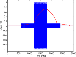
Also, there is a provision in the definition of a VU Meter’s ballistics for something called overshoot. When the signal is suddenly applied to the meter, the indicator jumps up to the level it’s trying to display, but it typically goes slightly over that level and then drops back to the correct level. That amount of overshoot is supposed to be no more than 1.5% of the actual signal level. (If you’re picky, you’ll notice that there is no overshoot plotted in Figures 10.15 and 10.16.)
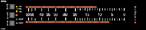
The good thing about VU Meters is that they show you the average level of the signal – so they’re great for recording to analog tape or for mastering purposes where you want to know the overall general level of the signal. However, they’re very bad at telling you the peak level of the signal – in fact, the higher the crest factor, the worse they are at telling you what’s going on. As we’ve already seen, there are many applications where we need to know exactly what the peak level of the signal is. Once upon a time, the only place where this was necessary was in broadcasting – because if you overload a transmitter, bad things happen. So, the people in the broadcasting world didn’t have much use for the VU Meter – they needed to see the peak of the program material, so the Peak Program Meter or PPM was developed in Europe around the same time as the VU Meter was in development in the US.
A PPM is substantially different from a VU Meter in many respects. These days it has many different incarnations – particularly in its scale, but the traditional one that most people think of is the UK PPM (also known as the BBC PPM). We’ll start there.
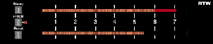
The UK PPM looks very different from a VU Meter – it has no decibel markings on it – just numbered indications from “Mark 0” up to “Mark 7.” In fact, the PPM is divided in decibels, they just aren’t marked there – generally, there are 4 decibels between adjacent marks – so from Mark 2 to Mark 3 is an increase of 4 dB. There are two exceptions to this rule – there are 6 decibels between Marks 0 and 1 (but note that Mark 0 is not marked). In addition, there are 2 decibels between Mark 7 and Mark 8 (which is also not marked).
Because we’re thinking now in terms of the peak signal level, the nominal level is less important than the maximum, however, PPM’s are calibrated so that Mark 4 corresponds to 0 dBu. Therefore if the PPM at the output stage on a mixing console read Mark 5 for a 1 kHz sine wave, then the output level is 1.228VRMS between pins 2 and 3 (because Mark 5 is 4 dB higher than Mark 4, making it +4 dBu).
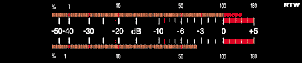
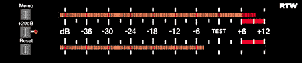
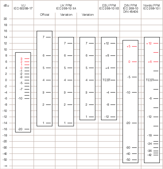
There are a number of other PPM Scales available to the buying public. In addition to the UK PPM, there’s the EBU PPM, the DIN PPM and the Nordic PPM. Each of these has a different scale as is shown in Table 10.1 and the corresponding Figure 10.19.
| Meter | Standard | Minimum Scale and | Maximum Scale and | Nominal Scale and |
| Corresponding Level | Corresponding Level | Corresponding Level | ||
| VU | IEC 60268–17 | –20 dB = –16 dBu | +3 dB = 7 dBu | 0 dB = 4 dBu |
| UK (BBC) PPM | IEC 268–10 IIA | Mark 1 = –14 dBu | Mark 7 = 12 dBu | Mark 4 = 0 dBu |
| EBU PPM | IEC 268–10 IIB | –12 dB = –12 dBu | +12 dB = 12 dBu | Test = 0 dBu |
| DIN PPM | IEC 268–10 / DIN 45406 | –50 dB = –44 dBu | +5 dB = 11 dBu | 0 dB = 6 dBu |
| Nordic PPM | IEC 268–10 I | –42 dB = –42 dBu | +12 dB = 12 dBu | Test (or 0 dB) = 0 dBu |
Let’s be complete control freaks and build the perfect PPM. It would show the exact absolute value of the voltage level of the signal all the time. The needle would dance up and down constantly and after about 3 seconds you’d have a terrible headache watching it. So, this is not the way to build a PPM. In fact, what is done is the ballistics are modified slightly so that the meter responds very quickly to a sudden increase in level, but it responds very slowly to a sudden drop in level – the decay time is much slower even than a VU Meter. You may notice that the PPM’s listed in Table 1 and Figure 10.19 are grouped into two “types” Type I and Type II. These types indicate the characteristics of the ballistics of the particular meter.
The attack time of a Type I PPM is defined using an integration time of 5 ms – which corresponds to a time constant of 1.7 ms. Therefore, a tone burst that is 10 ms long will result in the indicator being 1 dB lower than the correct level. If the burst is 5 ms long, the indicator will be 2 dB down, a 3 ms burst will result in an indicator that is 4 dB down. The shorter the burst, the more inaccurate the reading. (Note however, that this is significantly faster than the VU Meter.)
Again, unlike the VU meter, the decay time of a Type I PPM is not the reciprocal of the attack curve. This is defined by how quickly the indicator drops – in this case, the indicator will drop 20 dB in 1.4 to 2.0 seconds.
The attack time of a Type II PPM is identical to a Type I PPM.
The decay of a Type II PPM is somewhat different from its Type I cousin. The indicator falls back at a rate of 24 dB in 2.5 to 3.1 seconds. In addition, there is a “hold” function on the peak where the indicator is held for 75 ms to 150 ms before it starts to decay.
There’s one important thing to note in all of this discussion. This chapter assumes that we’re talking about professional equipment in a recording studio.
If you work with professional broadcast equipment, then the nominal level is different – in fact, it’s 4 dB higher than in a recording studio. 0 dB VU corresponds to +8 dBu and all of the other scales are higher to match.
If we’re talking about consumer–level equipment, either for recording or just for listening to things at home on your stereo, then the nominal 0 dB VU point (and all other nominal levels) corresponds to a level of -10 dBV or 0.316VRMS.
A digital meter is very similar to a PPM because, as we’ve already established, your biggest concern with digital audio is that the peak of the signal is never clipped. Therefore, we’re most interested in the peak or the amplitude of the signal.
As we’ve said before, the noise floor in a PCM digital audio signal is typically determined by the dither level which is usually at approximately one half of an LSB. The maximum digital level we can encode in a PCM digital signal is determined by the number of bits. If we’re assuming that we’re talking about a two’s complement system, then the maximum positive amplitude is a level that is expressed as a 0 followed by as many 1’s as are allowed in the digital word. For example, in an 8–bit system, the maximum possible positive level (in binary) is 01111111. Therefore, in a 16–bit system with 65536 possible quantization values, the maximum possible positive level is level number 32767. In a 24–bit system, the maximum positive level is 8388607. (If you’d like to do the calculation for this, it’s 2(n-1) -1 where n is the number of bits in the digital word.
Note that the negative–going signal has one extra LSB in a two’s complement system as is discussed in the chapter on digital conversion.
The maximum possible value in the positive direction in a PCM digital signal is called full scale because a sample that has that maximum value uses the entire scale that is possible to express with the digital word. (Note that we’ll see later that this definition is actually a lie – there are a couple of other things to discuss here, but we’ll get back to them in a minute.)
It is therefore evident that, in the digital world, there is some absolute maximum value that can be expressed, above which there is no way to describe the sample value. We therefore say that any sample that hits this maximum is “clipped” in the digital domain – however, this does not necessarily mean that we’ve clipped the audio signal itself. For example, it is highly unlikely that a single clipped sample in a digital audio signal will result in an audible distortion. In fact, it’s unlikely that two consecutively clipped samples will cause audible artifacts. The more consecutively clipped samples we have, the more audible the distortion. People tend to settle on 2 or 3 as a good number to use as a definition of a “clipped” signal.
If we look at a rectified signal in a two’s complement PCM digital domain, then the amplitude of a sample can be expressed using its relationship to a sample at full scale. This level is called dB FS or “decibels relative to full scale” and can be calculated using the following equation:
dB FS = 20 * log (sample value / maximum possible value)
Therefore, in a 16–bit system, a sine wave that has an amplitude of 16384 (which is also the value of the sample at the positive peak of the sine wave) will have a level of –6.02 dB FS because:
20 * log (16384 / 32767) = –6.02 dB FS
There’s just one small catch: I lied. There’s one additional piece of information that I’ve omitted to keep things simple. Take a close look at Figure 10.22. The way I made this plot was to create a sine wave and quantize it using a 4–bit system assuming that the sampling rate is 20 times the frequency of the sine wave itself. Although this works, you’ll notice that there are some quantization levels that are not used. For example, not one of the samples in the digital sine wave representation has a value of 0001, 0011 or 0101. This is because the frequency of the sine wave is harmonically related to the sampling rate. In order to ensure that more quantization levels are used, we have to use a sampling rate that is enharmonically related to the sampling rate. The technical definition of “full scale” uses a digitally–generated sine tone that has a frequency of 997 Hz. Why 997 Hz? Well, if you divide any of the standard sampling rates (32 kHz, 44.1 kHz, 48 kHz, 88.2 kHz, 96 kHz, etc...) by 997, you get a nasty number. The result is that you get a different quantization value for every sample in a second. You won’t hit every quantization value because the whole system starts repeating after one second – but, if your sine tone is 997 Hz and your sampling rate is 44.1 kHz, you’ll wind up hitting 44100 different quantization values. The higher the sampling rate, the more quantization values you’ll hit, and the less your error from full scale.
The other reason for using this system is to avoid signals that are actually higher than Full Scale without the system actually knowing. If you have a sine tone with a frequency that is harmonically related to the sampling rate, then it’s possible that the very peak of the wave is between two samples, and that it will always be between two samples. Therefore the signal is actually greater than 0 dB FS without you ever knowing it. With a 997 Hz tone, eventually, the peak of the wave will occur as close as is reasonably possible to the maximum recordable level.
This becomes part of the definition of full scale – the amplitude of a signal is compared to the amplitude of a 997 Hz sine tone at full scale. That way we’re sure that we’re getting as close as we can to that top quantization level.
There is one other issue to deal with: the definition of dB FS uses the RMS value of the signal. Therefore, a signal that is at 0 dB FS has the same RMS value as a 997 Hz sine wave whose peak positive amplitude reaches full scale. There are two main implications of this definition. The first has to do with the crest factor of your signal. Remember that the crest factor is a measurement of the relationship between the peak and the RMS value of the signal. In almost all cases, the peak value will be greater than RMS value (in fact, the only time this is not the case is a square wave in which they will be equal). Therefore, if a meter is really showing you the signal strength in dB FS, then it is possible that you are clipping your signal without your meter knowing. This is because the meter would be showing you the RMS level, but the peak level is much higher. It is therefore possible that you are clipping that peak without hitting 0 dB FS. This is why digital equipment also has an OVER indicator (check out Figure 10.23) to tell you that the signal has clipped. Just remember that you don’t necessarily have to go all the way up to 0 dB FS to clip.
Another odd implication of the dB FS definition is that, in the odd case of a square wave, you can have a level that is greater than 0 dB FS without clipping. The crest factor of a sine wave is 3.01 dB. This means that the RMS level of the sine tone is 3.01 dB less than its peak value. By comparison, the crest factor of a square wave is 0 dB, meaning that the peak and RMS values are equal. So what? Well, since dB FS is referenced to the RMS value of a sine wave whose maximum peak is at Full Scale (and therefore 3.01 dB less than Full Scale), if you put in a square wave that goes all the way up to Full Scale, it will have a level that is 3.01 dB higher than the Full Scale sine tone, and therefore a level of +3.01 dB FS. This is an odd thing for people who work a lot with digital gear. I, personally, have never seen a digital meter that goes beyond 0 dB. Then again, I don’t record square waves very often either, so it doesn’t really matter a great deal.
Chances are that the digital meter on whatever piece of equipment that you own really isn’t telling you the signal strength in dB FS. It’s more likely that the level shown is a sample–by–sample level measurement (and therefore not an RMS measurement) with a ballistic that makes the meter look like it’s decaying slowly. Therefore, in such a system, 0 dB on the meter means that the sample is at Full Scale.
I’m in the process of making a series of test tones so that you can check your meters to see how they display various signal levels. Stay tuned!

As far as I’ve been able to tell, there are no standards for digital meter ballistics or appearances, so I’ll just describe a typical digital meter. Most of these use what is known as a dot bar mode which actually shows two levels simultaneously. Looking at Figure 10.23, we can see that the meter shows a bar that extends to –24 dB. This bar shows the present level of the signal using ballistics that typically have roughly the same visual characteristics as a VU Meter. Simultaneously, there is a dot at the –8 dB mark. This indicates that the most recent peak hit –8 dB. This dot will be erased after approximately one second or so and be replaced by a new peak unless the signal peaks at a value greater than –8 dB in which case that value will be displayed by the dot. This is similar to a Type II PPM ballistic with the decay being replaced with simple erasure.
Many digital audio meters also include a function that gives a very accurate measurement of the maximum peak that has been hit since we’ve started recording (or playing). This value is usually called the margin and is typically displayed as a numerical value near the meter, but elsewhere on the display.
Finally, digital meters have a warning symbol to indicate that the signal has clipped. This warning is simply called over since all we’re concerned with is that the signal went over full scale – we don’t care how far over full scale it went. The problem here is that different meters use different definitions for the word “over.” As I’ve already pointed out, some meters keep track of the number of consecutive samples at full scale and point out when that number hits 2 or 3 (this is either defined by the manufacturer or by the user, depending on the equipment and model number – check your manual). On some equipment (particularly older gear), the “digital” meter is driven by the analog conversion of the signal and is therefore extremely inaccurate – again, check your manual. An important thing to note about these meters is that they rarely are aware that the signal has gone over full scale when you’re playing back a digital signal, or if you’re using an external analog to digital to convertor – so be very careful.
From the time the sound arrives at the diaphragm of your microphone to the time the signal gets recorded, it has to travel a very perilous journey, usually through a lot of wire and components that degrade the quality of the signal every step of the way. One of the best ways to minimize this degradation is to ensure that you have an optimal gain structure throughout your recording chain, taking into account the noise and distortion characteristics of each component in the signal path. This sounds like a monumental task, but it really hinges on a couple of very simple concepts.
The first basic rule (that you’ll frequently have to break but you’d better have a good reason...) is that you should make the signal as loud as you can as soon as you can. For example, consider the example of a microphone connected through a mic preamp into a DAT machine. We know that, in order to get the best quality digital conversion of the signal, its maximum should be just under 0 dB FS. Let’s say that, for the particular microphone and program material, you’ll need 40 dB of gain to get the signal up to that level at the DAT machine. You could apply that gain at the mic preamp or the analog input of the DAT recorder. Which is better? If possible, it’s best to get all of the gain at the mic preamp. Why? Consider that each piece of equipment adds noise to the signal. Therefore, if we add the gain after the mic preamp, then we’re applying that gain to the signal and the noise of the microphone preamp. If we add the gain at the input stage of the mic preamp, then its inherent noise is not amplified. For example, consider the following equations:
| (signal + noise) * gain | (signal * gain) + noise | |
| (signal * gain) + (noise * gain) | But: | |
| High signal level, high noise level | High signal level, low noise level | |
NOT WRITTEN YET
Before we talk about the issue of how to setup a playback system, we have to discuss the issue of standard operating levels. We have already seen that our ears have different sensitivities to different frequencies at different levels. Basically, at low listening levels, we can’t hear low-end material as easily as mid-band content. The louder the signal gets, the “flatter” the frequency response of our ears. In the practical world, this means that if I do a mix at a low level, then I’ll mix the bass a little hot because I can’t hear it. If I turn it up, it will sound like there’s more bass in the mix, because my ears have a different response.
Therefore, in order to ensure that you (the listener) hear what I (the mixing engineer) hear, one of the first things I have to specify is how loud you should turn it up. This is the reason for a standard operating level. That way, if you say “there’s not enough bass” I can say “you’re listening at too low a level” – unless you aren’t, then we have to talk about issues of taste. This subject will not be addressed in this book.
The film and television industries have an advantage that the music people don’t. They have international standards for operating levels. What this means is that a standard operating level on the recording medium and in the equipment will result in a standard acoustic level at the listening position in the mixing studio or theatre. Of course, we typically listen to the television at lower levels than we hear at the movie theatre, so these two levels are different.
Tables 10.3 shows the standard operating levels for film and television sound work. It also includes an approximate range for music mixing, although this is not a standard level.
| Medium | Signal level | Signal level | Signal level | Acoustic level |
| Film | -20 dB FS | 0 dB VU | +4 dBu | 85 dBspl |
| Television | -20 dB FS | 0 dB VU | +4 dBu | 79 dBspl |
| Music | -20 dB FS | 0 dB VU | +4 dBu | 79 - 82 dBspl |
It is important to note that the values in Table 10.3 are for a single loudspeaker measured with an SPL meter with a C-weighting and a slow response. So, for example, if you’re working in 5.1 surround for film, pink noise at a level of 0 dB VU sent to the centre channel only will result in a level of 85 dBspl at the mixing position. The same should be true of any other main channel.
Dolby has a slightly different recommendation in that, for film work, they suggest that each surround channel (which may be sent to multiple loudspeakers) should produce a standard level of 82 dBspl. This difference is applicable only to “film-style mixing rooms” [Dolby, 2000].
Furthermore, the EBU has a slightly different recommendation. In Technical Document 3276 [?][?], they specify that the “Alignment Signal Level” should be a pink noise signal with an RMS value of -18 dBFS on each channel. That signal should produce an acoustic level that is determined by the number of channels you have using Equation 10.1.
 | (10.1) |
Where LLISTref is the reference listening level in dB(A) (using an RMS, slow) at the listening position for each channel, each produced by a single loudspeaker, and where n is the number of channels. Therefore, for 2 channels, the level for each channel should be 82 dB(A). For a 5-channel configuration, the level for each channel should be 78 dB(A).
Before we go any further, we have to look at a commonly-confused issue in monitoring, particularly since the popularization of so-called 5.1 systems.
In a 5.1-channel mix, we have 5 main full-range channels, Left, Centre, Right, Left Surround and Right Surround. In addition, there is a channel which is band-limited from 0 to 120 Hz called the LFE or Low Frequency Effects channel.
In the listening room in the real world, we have a number of loudspeakers:
Of course, the situation I just described for the listening environment is not the optimal situation, but it’s a reasonable description of the real world. We’ll look at the ideal situation below.
If we look at a very simple configuration, then the L, R, C, LS and RS signals are connected directly to the L, R, C, LS and RS loudspeakers respectively, and the LFE channel is connected to the subwoofer. In most cases, however, this is not the only configuration. In larger listening rooms, we typically see more than two surround loudspeakers and more than one subwoofer. In smaller systems, people have been told that they don’t need 5 large speakers, because all the bass can be produced by the subwoofer using a bass management system described below, consequently, the subwoofer produces more than just the LFE channel.
So, it is important to remember that delivery channels are not directly equivalent to loudspeakers. It is an LFE channel – not a subwoofer channel.
Once upon a time, people who bought a stereo system bought two identical loudspeakers to make the sound they listened to. If they couldn’t spend a lot of money, or they didn’t have much space, they bought smaller loudspeakers which meant less bass. (This isn’t necessarily a direct relationship, but that issue is dealt with in the section on loudspeaker design... We’ll assume that it’s the truth for this section.)
Then, one day I walked into my local stereo store and heard a demo of a new speaker system that just arrived. The two loudspeakers were tiny little things - two cubes about the size of a baseball stuck together on a stand for each side. The sound was much bigger than these little speakers could produce... there had to be a trick. It turns out that there was a trick. The Left and Right channels from the CD were being fed to a crossover system where all the low-frequency information was separated from the high-frequency information, summed and sent to a single low-frequency driver sitting behind the couch I was sitting on. The speakers I could see were just playing the mid- and high-frequency information... all the low-end came from under the couch.
This is the concept behind bass management or bass redirection. If you have a powerful-enough dedicated low frequency loudspeaker, then your main speakers don’t need to produce that low frequency information. There are lots of arguments for and against this concept, and I’ll try to address a couple of these later, but for now, let’s look at the layout of a typical bass management system.
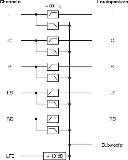
Figure 10.26 shows a block diagram for a typical bass management scheme. The five main channels are each filtered through a high-pass filter with a crossover frequency of approximately 80 Hz before being routed to their appropriate loudspeakers. These five channels are also individually filtered through low-pass filters with the same crossover frequency, and the outputs of the these filters is routed to a summing buss. In addition, the LFE channel input is increased in level by 10 dB before being added to the same buss. The result on this summing buss is sent to the subwoofer amplifier.
There is an important item to notice here – the 10 dB gain on the LFE channel. Why is this here? Well, consider if we send a full-scale signal to all channels. The single subwoofer is being asked to balance with 5 other almost-full-range loudspeakers, but since it is only one speaker competing with 5 others, we have to boost it to compensate. We don’t need to do this to the outputs resulting from the bass management system because the five channels of low-frequency information are added, and therefore boost themselves in the process. The reason this is important will be obvious in the discussion of loudspeaker level calibration below.
There are some basic rules to follow in the placement of loudspeakers in the listening space. The first and possibly most important rule of thumb is to remember that all loudspeakers should be placed at ear-level and aimed at the listening position. This is particularly applicable to the tweeters in the loudspeaker enclosure. Both of these simple rules are due to the fact that loudspeakers beam – that is to say that they are directional at high frequencies. In addition, you want your reproduced sound stage to be on your horizon, therefore the loudspeakers should be at your height. If it is required to place the loudspeakers higher (or lower) than the horizontal plane occupied by your ears, they should be angled downwards (or upwards) to point at your head.
The next issue is one of loudspeaker proximity to boundaries. As we discussed placing a loudspeaker immediately next to a boundary such as a wall will result in a boost of the low frequency components in the device. In addition a loudspeaker placed against a wall will couple much better to room modes in the corresponding dimension, resulting in larger resonant peaks in the room response. As a result, it is typically considered good practice to place loudspeakers on stands at least 1 m from any rigid surface. Of course, there are many situations where this is simply not possible. In these cases, correction of the loudspeaker’s response should be considered, either through post-crossover gain manipulation as is possible in many active monitors, or using equalization.
There are a couple of other issues to consider in this regard, some of which are covered below in Section 10.2.4.
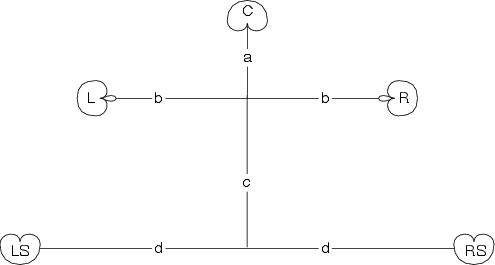
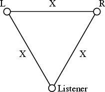
A two-channel playback system (typically misnamed “stereo”) has a standard configuration. Both loudspeakers should be equidistant from the listener and at angles of -30∘ and 30∘ where 0∘ is directly forward of the listener. This means that the listener and the two loudspeakers form the points of an equilateral triangle as shown in Figure 10.27, producing a loudspeaker aperture of 60∘.
Note that, for all discussions in this book, all positive angles are assumed to be on the right of centre forward, and all negative angles are assumed to be left of centre forward.
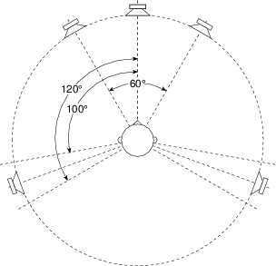
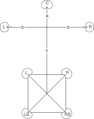
In the case of 5.1 surround sound playback, we are actually assuming that we have a system comprised of 5 full-range loudspeakers and no subwoofer. This is the recommended configuration for music recording and playback[Dolby, 2000] whereas a true 5.1 configuration is intended only for film and television sound. Again, all loudspeakers are assumed to be equidistant from the listener and at angles of 0∘, ±30∘ and with two surround loudspeakers symmetrically placed at an angle between ±100∘ and ±120∘. This configuration is detailed in ITU-R BS.775.1[ITU, 1994] (usually called “ITU775” or just “775” in geeky conversation... say all the numbers... “seven seven five” if you want to be immediately accepted by the in-crowd) and shown in Figure 10.28. If you have 25 Swiss Francs burning a hole in your pocket, you can order this document as a pdf or hardcopy from www.itu.ch. Note that the configuration has 3 different loudspeaker apertures, 30∘ (with the C/L and C/R pairs), approximately 80∘ (L/LS and R/RS) and approximately 140∘ (LS/RS).
How to set up a 5-channel system using only a tape measure
It’s not that easy to set up a 5-channel system using only angles unless you have a protractor the size of your room. Luckily, we have trigonometry on our side, which means that we can actually do the set up without ever measuring a single angle in the room. Just follow the step-by-step instructions below.
Step 1. Mark the listener’s location in the room and determine the desired distance to the loudspeakers (we’ll call that distance X ) Try to keep your loudspeakers at least 2 m from the listening position and no less than 1 m from any wall.
Step 2. Make an equalateral triangle marking the listener’s location, the Left and the Right loudspeakers as shown in the figure on the right. See Figure 10.29.
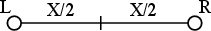
Step 3. Find the halfway point between the L and R loudspeakers and mark it. See Figure 10.30.
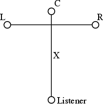
Step 4. Find the location of the C speaker using the halfway mark you just made, the listener’s location and the distance X. See Figure 10.31.
Step 5. Marks the locations for the LS and RS loudspeakers using the triangle measurements shown on the right. See Figure 10.32.
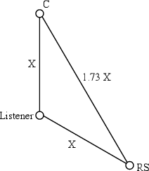
Step 6. Double check your setup by measuring the distance between the LS and RS loudspeakers. It should be 1.73X. (Therefore the C, LS and RS loudspeakers should make an equilateral triangle.) See Figure 10.33.

7. If the room is small, put the sub in the corner of the room. If the room is big, put the sub under the centre loudspeaker. Alternately, you could just put the sub where you think that it sounds best.
Room Orientation
There is a minor debate between opinions regarding the placement of the monitor configuration within the listening room. Usually, unless you’ve spent lots of money getting a listening room or control room designed from scratch, you’re probably going to be in a room that is essentially rectangular. This then raises two important questions:
Most people don’t think twice about the answer to the first question – of course you use the room symmetrically. The argument for this logic is to ensure a number of factors:
Therefore, your left / right pairs of speakers will “sound the same” (this also means the left surround / right surround pair) and your imaging will not pull to one side due to asymmetrical reflections.
Then again, the result of using a room symmetrically is that you are sitting in the dead centre of the room which means that you are in one of the worst possible locations for hearing room modes – the nulls are at a minimum and the antinodes are at a maximum at the centre of the room. In addition, if you listen for the fundamental axial mode in the width of the room, you’ll notice that your two ears are in opposite polarities at this frequency. Moving about 15 to 20 cm to one side will alleviate this problem which, once heard once, unfortunately, cannot be ignored.
So, it is up to your logic and preference to decide on whether to use the room symmetrically.
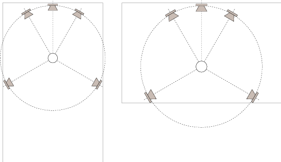
The second question of width vs. depth depends on your requirements. Figure 10.34 shows that the choice of room orientation has implications on the maximum distance to the loudspeakers. Both floorplans in the diagram show rooms of identical size with a maximum loudspeaker distance for an ITU775 configuration laid on the diagram. As can be seen, using the room as a wide, but shallow space allows for a much larger radius for the loudspeaker placement. Of course, this is a worst-case scenario where the loudspeakers are placed against boundaries in the room, a practice which is not advisable due to low-frequency boost and improved coupling to room modes.
From the very beginning, it was recognized that the 5.1 standard was a compromise. In a perfect system you would have an infinite number of loudspeakers, but this causes all sorts of budgetary and real estate issues... So we all decided to agree that 5 channels wasn’t perfect, but it was pretty good. There are people with a little more money and loftier ideals than the rest of us who are pushing for a system based on the MIBEIYDIS system (more-is-better-especially-if-you-do-it-smarter).
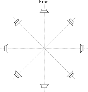
One of the most popular of these systems uses the standard 5.1 system as a starting point and expands on it. Dubbed 10.2 and developed by Tomlinson Holman (the TH in THX) this is actually a 12.2 system that uses a total of 16 loudspeakers.
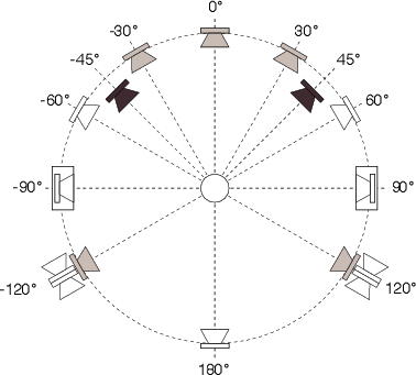
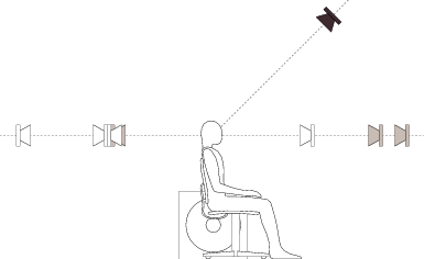
There are a couple of things to discuss about this configuration. Other than the sheer number of loudspeakers, the first big difference between this configuration and the standard ITU775 standard is the use of elevated loudspeakers. This gives the mixing engineer two possible options. If used as a stereo pair, it becomes possible to generate phantom images higher than the usual plane of presentation, giving the impression of height. If diffuse sound is sent to these loudspeakers, then the mix relies on our impaired ability to precisely localize elevated sound sources and therefore can give a better sense of envelopment than is possible with a similar number of loudspeakers distributed in the horizontal plane.
You will also notice that there are pairs of back-to-back loudspeakers placed at the ±90∘ positions. These are what are called diffuse radiators (although, technically speaking, they aren’t diffuse radiators...) and are actually wired to create a dipole radiator. In essence, you simply send the same signal to both loudspeakers in the pair, inverting the polarity of one of the two. This produces the dipole effect and, in theory, cancels all direct sound arriving at the listener’s location. Therefore, the listener receives only the reflected sound from the front and rear walls predominantly, creating the impression of a more diffuse sound than is typically available from the direct sound from a single loudspeaker.
Finally, you will note from the designation “10.2” that this system calls for two subwoofers. This follows the recommendations of a number of people [Martens, 1999][?] who have done research proving that uncorrelated signals from two subwoofers can result in increased envelopment at the listening position. The position of these subwoofers should be symmetrical, however more details will be discussed below.
See Section 10.5.2.
NOT WRITTEN YET
NOTES
Better to have many full-range speakers than 1 subwoofer
Floyd Toole’s idea of room mode cancellation through multiple correlated subwoofers
David Greisinger’s 2 decorrelated subwoofers driven by 1 channel
Bill Marten’s 2 subwoofer channels.
The calibration of your monitoring system is possibly one of the most significant factors that will determine the quality of your mixes. As a simple example, if you have frequency-independent level differences between your two-channel monitors, then your centre position is different from the rest of the world’s. You will compensate for your problem, and consequently create a problem for everyone else resulting in complaints that your lead vocals aren’t centered.
Unfortunately, it is impossible to create the perfect monitor, so you have to realize the limitations of your system and learn to work within those constraints. Essentially, the better you know the behaviour of your monitoring system, the more you can trust it, and therefore the more you can be trusted by the rest of us.
There is a document available from the ITU that outlines a recommended procedure for doing listening tests on small-scale impairments in audio systems [itu, 1997]. Essentially, this is a description of how to do the listening test itself, and how to interpret the results. However, there is a section in there that describes the minimum requirements for the reproduction system. These requirements can easily be seen as a minimum requirement for a reference monitoring system, and so I’ll list them here to give you an idea of what you should have in front of you at a recording or mixing session. Note that these are not standards for recording studios, I’m just suggesting that their a good set of recommendations that can give you an idea of a “good” playback system.
Note that all of the specifications listed here are measured in a free field (an anechoic chamber), 1 m from the acoustic centre of the loudspeaker.
Frequency Response
The on-axis frequency response of the loudspeaker should be measured in one-third octave bands using pink noise as a source signal. The response should not be outside the range of ±2 dB within the frequency range of 40 Hz to 16 kHz. The frequency response measured at 10∘ off-axis should not differ from the on-axis response by more than 3 dB. The frequency response measured at 30∘ off-axis should not differ from the on-axis response by more than 4 dB [itu, 1997].
All main loudspeakers should be matched in on-axis frequency response within 1 dB in the frequency range of 250 Hz to 2 kHz [itu, 1997].
Directivity Index
In the frequency range of 500 Hz to 10 kHz, the directivity index, C, of the loudspeakers should be within the limit 6 dB ≤ C ≤ 12 dB and “should increase smoothly with frequency” [itu, 1997].
Non-linear Distortion
Put one loudspeaker in an anechoic chamber and put your microphone 1 m in front of it, on axis. Send a sinusoidal tone between 40 Hz and 250 Hz to a loudspeaker that measures 90 dBspl at the microphone. If there is any distortion, then harmonics will be produced. None of those individual harmonics may be greater than 60 dBspl at the listening position (i.e. -30 dB relative to the 90 dBspl of the fundamental)[itu, 1997]. This also, means that you can have all harmonics present, as long as they are individually lower than 60 dBspl.
If the fundamental frequency of the input sinusoid is between 250 Hz and 16 kHz, then the same is true, but the threshold is 50 dBspl instead [itu, 1997].
Transient Fidelity
If you send a sine wave at any frequency to your loudspeaker and then stop the sine, it should not take more than 5 time periods of the frequency for the output to decay to 1/e (approximately 0.37 or -8.69 dB) of the original level [itu, 1997].
Time Delay
The delay difference between any two loudspeakers should not exceed 100 μs [itu, 1997]. (Note that this does not include propagation delay differences at the listening position.)
Dynamic Range
You should be able to play a continuous signal with a level of at least 108 dBspl for 10 minutes without damaging the loudspeaker and without overloading protection circuits [itu, 1997].
The equivalent acoustic noise produced by the loudspeaker should not exceed 10 dBspl, A-weighted [itu, 1997] WHAT IS EQUIVALENT ACOUSTIC NOISE?.
So, you’ve bought a pair of loudspeakers following the recommendations of all the people you know (but you bought the ones you like anyway...) you bring them to the studio and carefully position them following all the right rules. Now you have to make sure that the outputs levels of the two loudspeakers is matched. How do you do this?
You actually have a number of different options here, but we’ll just look at a couple, based on the assumption that you don’t have access to really serious (and therefore REALLY expensive) measurement equipment.
SPL Meter Method
One of the simplest methods of loudspeaker calibration is to use pink noise as your signal and an SPL meter as your measurement device. If an SPL meter is not available (a cheap one is only about $50 at Radio Shack... go treat yourself...) then you could even get away with an omnidirectional condenser microphone (the smaller the diaphragm, the better) and the meter bridge of your mixing console.
Send the pink noise signal to the amplifier (or the crossover input if you’re using active crossovers) for one of your loudspeakers. The level of the signal should be 0 dB VU (or +4 dBu).
Place the SPL meter at the listening position pointing straight up. If you are holding the meter, hold it as far away from your body as you can and stand to the side so that the direct sound from the loudspeaker to the meter reflects off your body as little as possible (yes, this will make a difference). The SPL meter should be set to C-weighting and a slow response.
Adjust your amplifier gain so that you get 85 dBspl on the meter. (Feel free to use a different value if you think that you have a really good excuse. The 85 dBspl reference value is the one used by the film industry. Television people use 79 dBspl and music people can’t agree on what value to use.)
Repeat this procedure with the other loudspeaker.
Remember that you are measuring one loudspeaker at a time – you should 85 dBspl from each loudspeaker, not both of them combined.
A word of warning: It’s possible that your listening position happens to be in a particular location where you get a big resonance due to a room mode. In fact, if you have a smaller room and you’ve set up your room symmetrically, this is almost guaranteed. We’ll deal with how to cope with this later, but you have to worry about it now. Remember that the SPL meter isn’t very smart – if there’s a big resonance at one frequency, that’s basically what you’re measuring, not the full-band average. If your two loudspeakers happen to couple differently to the room mode at that frequency, then you’re going to have your speakers matched at only one frequency and possibly no others. This is not so good.
There are a couple of ways to avoid this problem. You could change the laws of physics and have room modes eliminated in your room, but this isn’t practical. You could move the meter around the listening position to see if you get any weird fluctuations because many room modes produce very localized problems. However, this may not tell you anything because if the mode is a lower frequency, then the wavelength is very long and the whole area will be problematic. Your best bet is to use a measurement device that shows you the frequency response of the system at the listening position, the simplest of which is a real-time analyzer. Using this system, you’ll be able to see if you have serious problems in localized frequency bands.
Real-Time Analyzer Method
If you’ve got a real-time analyzer (or RTA) lying around, you could be a little more precise and get a little more information about what’s happening in your listening room at the listening position. Put an omnidirectional microphone with a small diaphragm at the listening position and aim it at the ceiling. The output should go to the RTA.
Using pink noise at a level of +4 dBu sent to a single loudspeaker, you should see a level of 70 dBspl in each individual band on the RTA [Owinski, 1998]. Whether or not you want to put an equalizer in the system to make this happen is your own business (this topic is discussed a little later on), but you should come as close as you can to this ideal with the gain at the front of the amplifier.
Other methods
There are a lot of different measurement tools out there for doing exactly this kind of work, however, they’re not cheap, and if they are, they may not be very reliable (although there really isn’t a direct correlation between price and system reliability...) My personal favourites for electroacoustic measurements are a MLSSA system from DRA Laboratories, and a number of solutions from Brüel & Kjær, but there’s lots of others out there.
Just be warned, if you spend a lot of money on a fancy measurement system, you should probably be prepared to spend a lot of time learning how to use it properly. My experience is that the more stuff you can measure, the more quickly and easily you can find the wrong answers and arrive at incorrect conclusions.
The method for calibrating a 5-channel system is no different than the procedure described above for a two-channel system, you just repeat the process three more times for your Centre, Left Surround and Right Surround channels. (Notice that I used the word “channels” there instead of “loudspeakers” because some studios have more than two surround loudspeakers. For example, if you do have more than one Left Surround loudspeaker, then your Left Surround loudspeakers should all be matched in level, and the total output from all of them combined should be equal to the reference value.)
The only problem that now arises is the question of how to calibrate the level of the subwoofer, but we’ll deal with that below.
The same procedure holds true for calibration of a 10.2 system. All channels should give you the same SPL level (either wide band with an SPL meter or narrow band with an RTA) at the listening position. The only exception here is the diffuse radiators at ±90∘. You’ll probably notice that you won’t get as much low frequency energy from these loudspeakers at the listening position due to the cancellation of the dipole. The easiest way to get around this problem is to band-limit your pink noise source to a higher frequency (say, 250 Hz or so...) and measure one of your other loudspeakers that you’ve already calibrated (Centre is always a good reference). You’ll notice that you get a lower number because there’s less low-end – write that number down and match the dipoles to that level using the same band-limited signal.
Again, the same procedure holds for an Ambisonics configuration.
Here’s where things get a little ugly. If you talk to someone about how they’ve calibrated their subwoofer level, you’ll get one of five responses:
Oddly enough, it’s possible that the first three of these responses actually mean exactly the same thing. This is partly due to an issue that I pointed out earlier in Section 10.2.3. Remember that there’s a 10 dB gain applied to the LFE input of a multichannel monitoring system for the remainder of this discussion.
The objective with a subwoofer is to get a low-frequency extension of your system without exaggerating the low-frequency components. Consequently, if you send a pink-noise signal to a subwoofer and look at its output level in a one-third octave band somewhere in the middle of its response, it should have the same level as a one-third octave band in the middle of the response of one of your other loudspeakers. Right? Well.... maybe not.
Let’s start by looking at a bass-managed signal with no signal sent to the LFE input. If you send a high-frequency signal to the centre channel and sweep the frequency down (without changing the signal level) you should see not change in sound pressure level at the listening position. This is true even after the frequency has gotten so low that it’s being produced by the subwoofer. If you look at Figure 10.26 you’ll see that this really is just a matter of setting the gain of the subwoofer amplifier so that it will give you the same output as one of your main channels.
What if you are only using the LFE channel and not using bass management? In this case, you must remember that you only have one subwoofer to compete with 5 other speakers, so the signal has been boosted by 10 dB in the monitoring box. This means that if you send a pink noise to the subwoofer and monitor it in a narrow band in the middle of its range, it should be 10 dB louder than a similar measurement done with one of your main channels. This extra 10 dB is produced by the gain in the monitoring system.
Since the easiest way to send a signal to the subwoofer in your system is to use the LFE input of your monitoring box, you have to allow for this 10 dB boost in your measurements.
Again, you can do your measurements with any appropriate system, but we’ll just look at the cases of an SPL meter and an RTA.
SPL Meter Method
We will assume here that you have calibrated all of your main channels to a reference level of 85 dBspl using + 4 dBu pink noise.
Send pink noise at +4 dBu, band-limited from 20 to 80 Hz, to your subwoofer through the LFE input of your monitor box. Since the pink noise has been band-limited, we expect to get less output from the subwoofer than we would get from the main channels. In fact, we expect it to be about 6 dB less. However, the monitoring system adds 10 dB to the signal, so we should wind up getting a total of 89 dBspl at the listening position, using a C-weighted SPL meter set to a slow response.
Note that some CD’s with test signals for calibrating loudspeakers take the 10 dB gain into account and therefore reduce the level of the LFE signal by 10 dB to compensate. If you’re using such a disc instead of producing your own noise, then be sure to find out the signal’s level to ensure that you’re not calibrating to an unknown level...
If you choose to send your band-limited pink noise signal through your bass management circuitry instead of through the LFE input, then you’ll have to remember that you do not have the 10 dB boost applied to the signal. This means that you are expecting a level of 79 dBspl at the listening position.
The same warning about SPL meters as was described for the main loudspeakers holds true here, but more so. Don’t forget that room modes are going to wreak havoc with your measurements here, so be warned. If all you have is an SPL meter, there’s not really much you can do to avoid these problems... just be aware that you might be measuring something you don’t want.
Real-Time Analyzer Method
If you’re using an RTA instead of an SPL meter, your goal is slightly easier to understand. As was mentioned above, the goal is to have a system where the subwoofer signal routed through the LFE input is 10 dB louder in a narrow band than any of the main channels. So, in this case, if you’ve aligned your main loudspeakers to have a level of 70 dBspl in each band of the RTA, then the subwoofer should give you 80 dBspl in each band of the RTA. Again, the signal is still pink noise with a level of +4 dBu and band-limited from 20 Hz to 80 Hz.
Summary
| Source | Signal level | RTA | SPL Meter | |
| (per band) | ||||
| Main channel | -20 dB FS | 70 dBspl | 85 dBspl | |
| Subwoofer (LFE input) | -20 dB FS | 80 dBspl | 89 dBspl | |
| Subwoofer (main channel input) | -20 dB FS | 70 dBspl | 79 dBspl | |
Before we get into the issue of the characteristics of various microphone configurations, we have to look at the general idea of panning in two-channel and five-channel systems. Typically, panning is done using a technique called constant power pair-wise panning which is a system whose name contains a number of different issues which are discussed in this and the next chapter.
As you walk around the world, you are able to localize sound sources with a reasonable degree of accuracy. This basically means that if your eyes are closed and something out there makes a sound, you can point at it. If you try this exercise, you’ll also find that your accuracy is highly dependent on the location of the source. We are much better at detecting the horizontal angle of a sound source than its vertical angle. We are also much better at discriminating angles of sound sources in the front than at the sides of our head. This is because we are mainly relying on two basic attributes of the sound reaching our ears. These are called the interaural time of arrival difference (ITD’s) and the interaural amplitude difference (IAD’s).
When a sound source is located directly in front of you, the sound arrives at your two ears at the same time and at the same level. If the source moves to the right, then the sound arrives at your right ear earlier (ITD) and louder (IAD) than it does in your left ear. This is due to the fact that your left ear is farther away from the sound source and that your head gets in the way and shadows the sound on your left side.
Panning techniques rely on these same two differences to produce the simulation of sources located between the loudspeakers at predictable locations. If we send a signal to just one loudspeaker in a two-channel system, then the signal will appear to come from the loudspeaker. If the signal is produced by both loudspeakers at the same level and the same time, then the apparent location of the sound source is at a point directly in front of the listener, halfway between the two loudspeakers. Since there is no loudspeaker at that location, we call the effect a phantom image.
The exact location of a phantom image is determined by the relationship of the sound produced by the two loudspeakers. In order to move the image to the left of centre, we can either make the left channel louder, earlier, or simultaneously louder and earlier than the right channel. This system uses essentially the same characteristics as our natural localization system, however, now, we are talking about interchannel time differences and interchannel amplitude differences.
Almost every pan knob on almost every mixing console in the world is used to control the interchannel amplitude difference between the output channels of the mixer. In essence, when you turn the pan knob to the left, you make the left channel louder and the right channel quieter, and therefore the phantom image appears to move to the left. There are some digital consoles now being made which also change the interchannel time differences in their panning algorithms, however, these are still very rare.
This panning of phantom images can be accomplished not only with a simple pan knob controlling the electrical levels of the two or more channels, we can also rely on the sensitivity pattern of directional microphones to produce the same level differences.
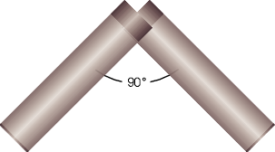
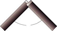
For example, let’s take two cardioid microphones and place them so that the two diaphragms are vertically aligned - one directly over the other. This vertical alignment means that sounds reaching the microphones from the horizontal plane will arrive at the two microphones simultaneously – therefore there will be no time of arrival differences in the two channels. consequently we call them coincident. Now let’s arrange the microphones such that one is pointing 45∘ to the left and the other 45∘ to the right, remembering that cardioids are most sensitive to a sound source directly in front of them.
If a sound source is located at 0∘, directly in front of the pair of microphones, then each microphone is pointing 45∘ away from the sound source. This means that each microphone is equally insensitive to the sound arriving at the mic pair, so each mic will have the same output. If each mic’s output is sent to a single loudspeaker in a stereo configuration then the two loudspeakers will have the same output and the phantom image will appear dead centre between the loudspeakers.
However, let’s think about what happens when the sound source is not at 0∘. If the sound source moves to the left, then the microphone pointing left will have a higher output because it is more sensitive to signals in directly in front of it. On the other hand, we’re moving further away from the front of the right-facing microphone so its output will become quieter. The result in the stereo image is that the left loudspeaker gets louder while the right loudspeaker gets quieter and the image moves to the left.
If we had moved the sound source towards the right, then the phantom image would have moved towards the right.
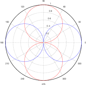
This system of two coincident 90∘ cardioid microphones is very commonly used, particularly in situations where it it important to maintain what is called mono compatibility. Since the signals arriving at the two microphones are coincident, there are no phase differences between the two channels. As a result, there will be no comb filtering effects if the two channels are summed to a single output as would happen if your recording is broadcast over the radio. Note that, if a pair of 90∘ coincident cardioids is summed, then the total result is a single, virtual microphone with a sort of weird subcardioid-looking polar plot, but we’ll discuss that later.
Another advantage of using this configuration is that, since the phantom image locations are determined only by interchannel amplitude differences, the image locations are reasonably stable and precise.
There are, however, some disadvantages to using this system. To begin with, all of your sound sources located at the centre of the stereo sound stage are located off-axis to the microphones. As a result, if you are using microphones whose off-axis response is less than desirable, then you may experience some odd colouration problems on your more important sources.
A second disadvantage to this technique is that you’ll find that, when your musicians are distributed evenly in front of the pair (as in a symphony orchestra, for example), you get sources sounding like they’re “clumping” in the middle of your sound stage. There are a number of different ways of thinking of why this is the case. One explanation is presented in Section 10.4.1. A simpler explanation is given by Jörg Wuttke of Schoeps Microphones. As he points out, a cardioid is one half omnidirectional and one half bidirectional. Therefore, a pair of coincident cardioids gives you a signal, half of which is a pair of coincident omnidirectionals. A pair of coincident omni’s will give you a completely mono signal which will image in the dead centre of your loudspeakers – therefore instruments tend to pull to this location.
As we’ll see in the next chapter, although a pair of coincident cardioid microphones does indeed give you good imaging characteristics, there are many problems associated with this technique. In particular, you will find that the overall sound stage in a two-channel stereo playback tends to “clump” to the centre quite a bit. in addition, there is no feeling of “spaciousness” that can be generated with phase or polarity differences between the two channels. Both of these problems can be solved by trading in your cardioids for a pair of bidirectional microphones. An arrangement of two bidirectionals in a coincident pair with one pointing 45∘ to the left and the other 45∘ to the right is commonly called a Blumlein pair, named after the man who patented two-channel stereo sound reproduction, Alan Blumlein.
The outputs of these two bidirectional microphones have some interesting characteristics that will be analyzed in the next chapter, however, we can look at the basic attributes of the configuration here. To begin with, in the area in front of the microphones, you have basically the same behaviour as we saw with the coincident cardioid pair. Changes in the angle of incidence of the sound source result in changes in the interchannel amplitude differences in the channels, resulting in simple pair-wise power panning. Note however, that this pair is more sensitive to changes in angle, so you will experience bigger swings in the location of sound sources with a Blumlein pair than with 90∘ cardioids.
Let’s consider what’s happening at the rear of a Blumlein pair. Since a bidirectional microphone has a rear lobe that is symmetrical to the front one, but with a negative polarity, then a Blumlein pair of microphones will have the same response in the rear as it does in the front with only two exceptions. Sources on the rear left of the pair image on the right and sources on the right image on the left. This is because the rear lobe of the left microphone is pointing towards the rear right of the pair, consequently, the left – right orientation of the sources is flipped.
The other consequence of placing sources in the rear of the pair is that the direct sound is entering the microphones in their negative lobes. As a result, the polarity of the signals is inverted. This will not be obvious for many sources such as wind and string instruments, but you may be able to make a case for the difference being audible on more percussive sounds.
The other major difference between the Blumlein technique and coincident cardioids occurs when sound sources are located on the sides of the pair. For example, in the case of a sound source located at 90∘ off-axis to the pair on the left, then the source will be positioned in the front lobe of the left microphone but the rear lobe of the right microphone. As a result, the outputs of the two microphones will be matched in level, but they will be opposite in polarity. This results in the same imaging characteristics as we get when we wire one loudspeaker ‘out of phase’ with the other – a very unstable, “phasey” sound that could even be considered to be located outside the loudspeakers.
The interesting thing about this configuration, therefore, is that sound sources in front of the pair (like an orchestra) image normally; we get a good representation of the reverberation and audience coming from the front and rear lobes of the microphones; and that the early reflections from the side walls probably come in the sides of the microphone pair, thus imaging “outside” the loudspeaker aperture.
There are many other advantages to using a Blumlein pair, but these will be discussed in the next chapter.
There are some disadvantages to using this configuration. To begin with, bidirectional microphones are not as available or as cheap as cardioid microphones. The second is that, if a Blumlein pair is summed to mono, then the resulting virtual microphone is a forward-facing bidirectional microphone. This might not be a bad thing, but it does mean that you get as much from the rear of the pair as you do from the front, which might result in a sound that is a little too distant sounding in mono.
There are many occasions where you will want to add some extra microphones out in the hall to capture reverberation with very little direct sound. This is helpful, particularly in sessions where you don’t have a lot of sound-check time, or when the hall has problems. (Typically, you can cover up acoustical problems by adding more microphones to smear things out.)
Many people like to use VERY widely spaced omni’s for this, but this technique really doesn’t make much sense. As we’ll see later, the further apart a pair of microphones are in a diffuse field (like a reverberant concert hall) the less correlated they are. If your microphones are stuck on opposite sides of the hall (this is not an uncommon practice) you basically get two completely uncorrelated signals. The result is that the reverberation (and the audience noise, if they’re there) sits in two discrete pockets in the listening room – one pocket for each loudspeaker. This gives the illusion of a very wide sound, but there is nothing holding the two sides together – it’s just one big hole in the middle.
So, how can we get a nice, wide hall sound, with an even spread and avoid picking up too much direct sound?
This is the goal of the ES (or Enhanced Surround) microphone technique developed by Wieslaw Woszczyk. The configuration is simply two cardioids with an included angle of 180∘ degrees (placed back-to-back) with one of the outputs reversed in polarity. Each microphone is panned completely to one channel.
This technique has a number of interesting properties. It was initially developed to make a microphone technique that was compatible with the old matrixed surround systems from Dolby. Since the information coming in the centre of this pair is opposite in polarity between the two mic’s, this info would come through a 2-4 matrix and wind up in the surrounds. Therefore you had control over your surround info in the matrix, with a smooth transition from surround to left and right as the sound came around to either side of the pair from the middle. Also, if you sum your mix to mono, this pair gives you the same output as if you had a bidirectional mic in the same location. Since the null of that bidirectional is probably facing the stage, you get reverb, and very little slap delay from the direct sound. Of course, it could be argued that you want less reverb in a mono mix, to keep things intelligible... but that’s a personal opinion.
If you do want to try this technique, I would highly recommend implementing it using a technique borrowed from an MS pair. Set up a coincident omnidirectional and bidirectional with the null of the bidirectional facing forwards (so the mic is facing sideways). Send the two signals through a standard MS matrix where the bidirectional is the M channel and the omni is the S channel. The result will be a perfectly matched ES pair with the benefits of negatively correlated low frequency (thanks to the low-end response of the omni).
We have seen above that left – right localization can be achieved with interchannel time differences instead of interchannel amplitude differences. Therefore, if a signal comes from both loudspeakers at the same level, but one loudspeaker is slightly delayed (no more than about a millisecond or so), then the phantom image will pull towards the earlier loudspeaker.
This effect can be achieved in DSP using simple digital delays, however, we can also get a similar effect using two omnidirectional microphones, spaced apart by some distance. Now, if a sound source is off to one side of the spaced pair, then the direct sound will arrive at one microphone before the other and therefore cause an interchannel time difference using distance as our delay line. In this case, the closer the sound source is to 90∘ to one side of the pair, the greater the time difference, with a maximum at 90∘.
There are a number of advantages to using this technique. Firstly, since we’re using omnidirectional microphones, we are probably using microphones with well-behaved off-axis frequency responses. Secondly, we will get a very extended low frequency response due to the natural frequency range characteristics of an omnidirectional microphone. Finally, the resulting sound, due to the angle- and frequency-dependent phase differences between the two channels will have “fuzzy” imaging characteristics. Sources will not be precisely located between the loudspeakers, but will have wider, more nebulous locations in the stereo sound stage. Of course, this may be a disadvantage if you’re aiming for really precise imaging.
There are, of course, some disadvantages to using this technique. Firstly, the imaging characteristics are imprecise as was discussed above. In addition, if your microphones are placed too close together, you will get a very mono-like sound, with an exaggerated low frequency content in the listening room due to the increased correlation at longer wavelengths. If the microphones are placed too far apart, then there will be no stable centre image at all, resulting in a hole-in-the-middle effect. In this case, all sound sources appear at or around the loudspeakers with nothing in between.
Coincident microphone techniques rely solely on interchannel amplitude differences to produce the desired imaging effects. Spaced techniques, in theory, produce only interchannel time differences. There is, however, a hybrid group of techniques that produce both interchannel amplitude and time of arrival differences. These are known as near-coincident techniques, using a pair of directional microphones with a small separation.
As was discussed above, a pair of coincident cardioid microphones provides good mono compatibility, good for radio broadcasts, but does not result in a good feeling of spaciousness. Spaced microphones are the opposite. Once upon a time, the French national broadcaster, the ORTF (L’Office de Radiodiffusion-Télévision Française) wanted to create a happy medium between these two worlds – to have a microphone configuration with reasonable mono compatibility and some spaciousness (or is that not much spaciousness and poor mono compatibility... I guess it depends if you’re a glass-is-half-full or a glass-is-half-empty person. I’m a glass-is-not-only-half-empty-but-now-it’s-also-dirty person, so I’m the wrong one to ask.)
The ORTF came up with a configuration that, it’s said, resembles the configuration of a pair of typical human ears. You take two cardioid microphones and place them at an angle of 110∘ and 17 cm apart at the capsules.
Not to be outdone, the Dutch national broadcaster, the NOS (Nederlandse Omroep Stichting), created a microphone configuration recommendation of their own. In this case, you place a pair of cardioid microphones with an angle of 90∘ and a separation of 30 cm.
As you would expect from the larger separation between the microphones, your mono compatibility in this case gets worse, but you get a better sense of spaciousness from the output.
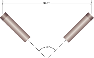
One of the problems with the ORTF and NOS configurations is that they both have their microphones aimed away from the centre of the stage. As a result, what are likely the more important sound sources are subjected to the off-axis response of the microphones. In addition, these configurations may create problems in halls with very strong sidewall reflections, since there is very little attenuation of these sources as a result of directional characteristics.
One option that resolves both of these problems is known as the Faulkner Technique, named after its inventor, Tony Faulkner. This technique uses a pair of bidirectional microphones, both facing directly forward and with a separation of about 20 cm. In essence, you can consider this configuration to be very similar to a pair of spaced omnidirectionals but with heavy attenuation of side sources, particularly sidewall reflections.
Spaced omnidirectional microphones have a nice, open spacious sound. The wider the separation, the more spacious, but if they get too wide, then you get a hole-in-the-middle. Also, you can wind up with some problems with sidewall reflections that are a little too strong, as was discussed in the section on the Faulkner technique.
The British record label Decca came up with a technique that solves all of these problems. They start with a very widely spaced pair of Neumann M50’s. This is an interesting microphone consisting of a 25 mm diameter omnidirectional capsule mounted on the face of a 40 mm plastic sphere. The omni capsule gives you a good low frequency response while the sphere gives you a more directional pattern in higher frequencies. (In recent years, many manufacturers have been trying to duplicate this by selling spheres of various sizes that can be attached to a microphone.)
The pair of omni’s is placed too far apart to give a stable centre image, but they provide a very wide and spacious sound. The centre image problem is solved by placing a third M50 placed between and in front of the pair. The output of this microphone is sent to both the left and right channels.
This configuration, known as a Decca Tree has been used by Decca for probably all of their orchestral recordings for many many years.
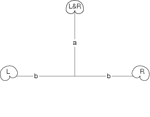
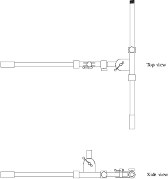
NOT WRITTEN YET
NOT WRITTEN YET
The Stereophonic Zoom by Michael Williams. Download this, read it and understand everything in it. You will not be sorry.
Note: Before reading this section, you should be warned that a thorough understanding of the material in Section 6.7 is highly recommended.
It is very important to remember that the exact location of a phantom image will be different for every listener. However, there have been a number of studies done which attempt to get an idea of roughly where most people will hear a sound source as we manipulate these parameters.
For two-channel systems, the study that is usually quoted was done by Gert Simonsen during his Master’s Degree at the Technical University of Denmark in Lyngby[Simonsen, 1984][Williams, 1990][Rumsey, 2001]. His thesis was constrained to monophonic sound sources reproduced through a standard two-channel setup. Modifications of the signals were restricted to basic delay and amplitude differences, and combinations of the two. According to his findings, some of which are shown in Table 10.5, in order to achieve a phantom image placement of 0∘ (or the centre-point between the two loudspeakers) both channels must be identical in amplitude and time. Increasing the amplitude of one channel by 2.5 dB (while maintaining the interchannel time relationship) will pull the phantom image 10∘ off-centre towards the louder speaker. The same result can be achieved by maintaining a 0.0 dB amplitude difference and delaying one channel by 0.22 ms. In this case, the image moves 10∘ away from the delayed loudspeaker. The amplitude and time differences for 20∘ and 30∘ phantom image placements are listed in Table 10.5 and represented in Figures 10.41 and 10.42.
| Image Position | ΔAmp. | ΔTime |
| 0∘ | 0.0 dB | 0.0 mS |
| 10∘ | 2.5 dB | 0.2 mS |
| 20∘ | 5.5 dB | 0.44 mS |
| 30∘ | 15.0 dB | 1.12 mS |
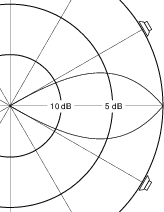
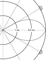
A similar study was done by the author at McGill University for a 5-channel configuration[Martin et al., 1999]. In this case, interchannel differences were restricted to either the amplitude or time domain without combinations for adjacent pairs of loudspeakers. It was found that different interchannel differences were required to move a phantom image to the position of one of the loudspeakers in the pair as are listed in Tables 10.6 and 10.7 Note that these values should be used with caution due to the large standard deviations in the data produced in the test. One of the principal findings of this research was the large variations between listeners in the apparent location of the phantom image. This is particularly true for side locations, and moreso for images produced with time differences.
| Pair (1/2) | 1 | 2 |
| C / L | 14 dB | 12 dB |
| L / LS | 9 dB | >16 dB |
| LS / RS | 9 dB | 9 dB |
| Pair (1/2) | 1 | 2 |
| C / L | >2.0 ms | 2.0 ms |
| L / LS | 1.6 ms | >2.0 ms |
| LS / RS | 0.6 ms | 0.6 ms |
Using the smoothed averages of the phantom image locations, polar plots can be generated to indicate the required differences to produce a desired phantom image position as are shown in Figures 10.43 and 10.44.
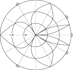
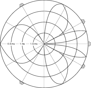
It is typically assumed that, when you’re sitting and listening to the the sound coming out of more than one loudspeaker, the total sound level that you hear is the sum of the sound powers, and not the sound pressures from the individual drivers. As a result, when you pan a single sound from one loudspeaker to another, you want to maintain a constant summed power, rather than a constant summed pressure.
The top plot in Figure 10.45 shows the two gain coefficients determined by the rotation of a pan knob for two output channels. Since the sum of the two gains at any given position is 1, this algorithm is called a constant amplitude panning curve. It works, but, if you take a look at the bottom plot in the same figure, you’ll see the problem with it. When the signal is panned to the centre position, there is a drop in the total summed power – in fact, it has dropped by half (or 3 dB) relative to an image located in one of the loudspeakers. Consequently, if this system was used for the panning in a mixing console, as you swept an image from left to centre to right, it would appear to get further away from you at the centre location because it appears to be quieter.
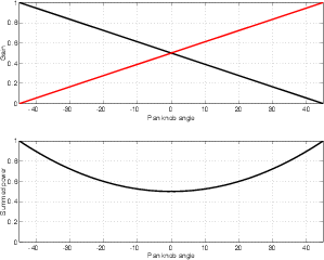
Consequently we have to use an algorithm which gives us a constant summed power as we sweep the location of the image from one loudspeaker to the other. This is accomplished by using modifying the gain coefficients as is shown in Figure 10.46.
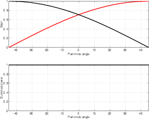
In order to understand the response of a signal from a pair of microphones (whether they’re alone, or part of a larger array) we must begin by looking at the differences in the outputs of the two devices.
Cardioids
Unless you only record pop music and you never use your imagination, all of the graphs shown above don’t really apply to what happens when you’re recording. This is because, usually your microphone isn’t pointing directly forward... you usually have more than one microphone and they’re usually pointing slightly to the left or right of forward, depending on your configuration. Therefore, we have to think about what happens to the sensitivity pattern when you rotate your microphone.
Figure 10.47 shows the sensitivity pattern of a cardioid microphone that is pointing 45∘ to the right. Notice that this plot essentially looks exactly the same as Figure 6.137, it’s just been pushed to the side a little bit.
Now let’s consider the case of a pair of coincident cardioid microphones pointed in different directions. Figure 10.49 shows the plots of two polar patterns for cardioid microphones point at -45∘ and 45∘, giving us an included angle (the angle subtended by the microphones) of 90∘ as is shown in Figure 10.48.
Figure 10.49 gives us two important pieces of information about how a pair of cardioid microphones with an included angle of 90∘ will behave. Firstly, let’s look at the vertical difference between the two curves. Since this plot essentially shows us the output level of each microphone for a given angle, then the distance between the two plots for that angle will tell us the interchannel amplitude difference. For example, at an angle of incidence (to the pair) of 0∘, the two plots intersect and therefore the microphones have the same output level, meaning that there is an amplitude difference of 0 dB. This is also true at 180∘, despite the fact that the actual output levels are different than they are at 0∘ – remember, we’re looking at the difference between the two channels and ignoring their individual output levels.
In order to calculate this, we have to find the ratio (because we’re thinking in decibels) between the sensitivities of the two microphones for all angles of incidence. This is done using Equation 10.2.
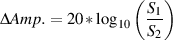 | (10.2) |
where
 | (10.3) |
where Ω is the angle of rotation of the microphone in the horizontal plane.
If we plot this difference for a pair of cardioids pointing at ±45∘, the result will look like Figure 10.50. Notice that we do indeed have a ΔAmp. of 0 dB at 0∘ and 180∘. Also note that the graph has positive and negative values on the right and left respectively. This is because we’re comparing the output of one microphone with the other, therefore, when the values are positive, the right microphone is louder than the left. Negative numbers indicate that the left is louder than the right.
Now, if you’re using this configuration for a two-channel recording, if you like, you can feel free to try and make a leap from here back to Table 10.5 to make some conclusion about where things are going to wind up being located in the reproduced sound stage. For example, if you believe that a signal with a ΔAmp. of 2.5 dB results in a phantom image location of 10∘, then you can go to the graph in Figure 10.50, find out where the graph crosses a ΔAmp. of 2.5 dB then find the corresponding angle of incidence. This then tells you that an instrument located at that angle to the microphone pair will show up at 10∘ off-centre between the loudspeakers. This is, of course, if you’re that one person in the world for whom Table 10.5 holds true (meaning you’re probably also 172.3 cm tall, you have 2.6 children and two thirds of a dog, you live in Boise, Idaho and that your life is exceedingly... well... average...)
We can do this for any included angle between the microphone pair, from 0∘ through to 180∘. There’s no point in going higher than 180∘ because we’ll just get a mirror image. For example, the response for an included angle of 190∘ is exactly the same as that for 170∘, just pointing towards the rear of the pair instead of the front.
Of course, if we actually do the calculation for an included angle of 0∘, we’re only going to find out that the sensitivities of the two microphones are matched, and therefore the ΔAmp. is 0 dB at all angles of incidence as is shown in Figure 10.51. This is true regardless of microphone polar pattern.
Note that, in the case of all included angles except for 0∘, the plot of ΔAmp. for cardioids goes to ±∞ dB because there will be one angle where one of the microphones has no output and because, on a decibel scale, something is infinitely louder than nothing.
Also note that, in the case of cardioids, every value of ΔAmp. is duplicated at another angle of incidence. For example, in the case of an included angle of 90∘, ΔAmp. = +10 dB at angles of incidence of approximately 70∘ and 170∘. This means that sound sources at these two angles of incidence to the microphone pair will wind up in the same location in the reproduced sound stage. Remember, however, that we don’t know the relative levels of these two sources because, all we know is their difference. It’s quite probable that one of these two locations will result in a signal that is much louder than the other, but that isn’t our concern just yet.
Also note that there is one included angle (of 180∘) that results in a response characteristic that is symmetrical (at least in each polarity) around the ∞ dB point.
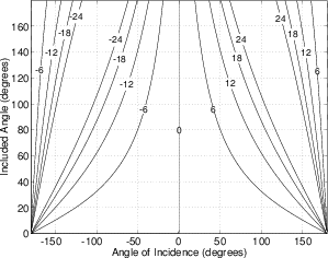
Subcardioids
Looking back at Figures 6.139 and 6.140 we can see that the lowest sensitivity from a subcardioid microphone is 6 dB below its on-axis sensitivity. As a result, unlike a pair of cardioid microphones, the ΔAmp. of a pair of subcardioid microphones cannot exceed the ±6 dB window, regardless of included angle or angle of incidence.
As can be seen in Figures 10.56 through 10.59, a pair of subcardioid microphones does have one characteristic in common with a pair of cardioid microphones in that there are two angles of incidence for every value of ΔAmp.
There is another aspect of subcardioid microphone pairs that should be remembered. As has already been discussed, in the case of subcardioids, it is impossible to have a value of ΔAmp. outside the ±6 dB window. Armed with this knowledge, take a look back at Tables 10.5, 10.6 and 10.7. You’ll note that in all cases of pair-wise panning, it takes more than 6 dB to swing a phantom image all the way into one of the two loudspeakers. Consequently, it is safe to say that, in the particular case of coincident subcardioid microphones, all of the the sound stage will be confined to a width smaller than the angle subtended by the two loudspeakers reproducing the two signals. As a result, if you want an image that is at least as wide as the loudspeaker aperture, you’ll have to introduce some time differences between the microphone outputs by separating them a little. This will be discussed further below.
Bidirectionals
The discussion of pairs of bidirectional microphones has to start with a reminder of two characteristics of their polar pattern. Firstly, the negative polarity of the rear lobe can never be forgotten. Secondly, as we will see below, it is significant to remember that, in the horizontal plane, this microphone has two angles which have a sensitivity of 0 (or -∞ dB).
Figure 10.60 shows the ΔAmp. of the absolute value of a pair of bidirectional microphones with an included angle of 90∘. In this case, the absolute value of the microphone’s sensitivity is used in order to avoid errors when calculating the logarithm of a negative number. This negative is the result of angles of incidence which produce sensitivities of opposite polarity in the two microphones. For example, in this particular case, at an angle of incidence of +90∘ (to the right), the right microphone sensitivity is positive while the left one is negative. However, it must be remembered that the absolute value of these two sensitivities are identical at this location.
A number of significant characteristics can be seen in Figure 10.60.
Firstly, note that there are now four angles of incidence where the ΔAmp. reaches -∞ dB. This is due to the fact that, in the horizontal plane, bidirectional microphones have two null points.
Secondly, note that the pattern in this plot is symmetrical around these infinite peaks, just as was the case with a pair of cardioid microphones at 180∘, apparently resulting in four angles of incidence which result in sound sources located at the same phantom image location. This, however, is not the case due to polarity differences. For example, although sound sources located at 30∘ and 60∘ (symmetrical around the 45∘ location) appear to result in identical sensitivities, the 30∘ location produces similar polarity signals whereas the 60∘ location produces opposite polarity signals.
Finally, it is significant to note that the response of the microphone pair is symmetrical front-to-back, with a left/right and a polarity inversion. For example, a sound source at +10∘ results in the same ΔAmp. as a sound source at -170∘, however, the rear source will be have a negative polarity in both channels. Similarly, a sound source at +60∘ will have the same ΔAmp. as a sound source at -120∘, however the former will be positive in the “right” channel and negative in the “left” whereas the opposite is the case for the latter.
Various other included angles for a pair of bidirectional microphones results in a similar pattern as was seen in Figure 10.60, with a “skewing” of the response curves. This can be seen in Figures 10.61 and 10.62.
It is also important to note that Figures 10.61 and 10.62 are mirror images of each other. This, however does not simply mean that the pair can be considered to be changed from “pointing” from the front to the side in this case. This is again due to the polarity differences between the two channels for specific various angles of incidence.
There is one final configuration worth noting in the specific case of bidirectional microphones; when the included angle is 180∘. As can be seen in Figure 10.63, this results in the absolute values of the sensitivities being matched at all angles of incidence. Remember however, that in this particular case, this means that the two channels are exactly matched and opposite in polarity – theoretically, you wind up with exactly the same signal as you would with one microphone split to two channels on the mixing console and the polarity switch (frequently incorrectly referred to as the “phase” switch) engaged on one of the two channels.
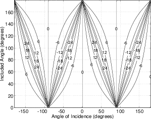
Hypercardioids
Not surprisingly, the response of a pair of hypercardioid microphones looks like a hybrid of the bidirectional and cardioid pairs. As can be seen in Figure 10.65, there are four infinite peaks in the value of ΔAmp., similar to bidirectional pairs, however the slope of the peaks are skewed further left and right as in the case of cardioids.
Again, similar to the case of bidirectional microphones, changing the included angle of the hypercardioids results in a further skewing of the response curve to one side or the other as can be seen in Figures 10.66 and 10.67.
Figure 10.68 shows the interesting case of hypercardioid microphones with an included angle of 180∘. In this case the maximum sensitivity point in the rear lobe of each microphone is perfectly aligned with the maximum sensitivity point in the other microphone’s front lobe. However, since the rear lobe has a sensitivity with an absolute value that is 6 dB lower than the front lobe, the value of ΔAmp. remains outside the ±6 dB window for the larger part of the 360∘ rotation.
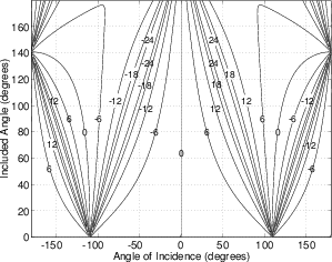
Spaced omnidirectionals
In the case of spaced omnidirectional microphones, it is commonly assumed that the distance to the sound source is adequate to ensure that the impinging sound can be considered to be a plane wave. In addition, it is also assumed that there is no difference in signal levels due to differences in propagation distance to the transducers. In reality, for widely spaced microphones and/or for sound sources closely located to any microphone, neither of these assumptions is correct, however they will be used for this discussion.
The difference in time of arrival of a sound at two spaced microphones is dependent both on the separation of the transducers d and the angle of rotation around the pair ϑ.
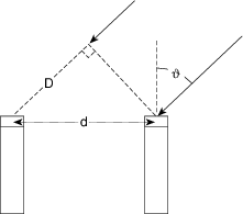
The additional distance, D, travelled by the sound wave to the further of the two microphones, shown in Figure 10.70, can be calculated using Equation 10.4.
 | (10.4) |
where d is the distance between the microphone capsules in cm.
The additional time ΔTime required for the sound to travel this distance is calculated using Equation 10.5.
 | (10.5) |
where ΔTime is the interchannel time difference in ms, ϑ is the angle of incidence of the sound source to the pair, and c is the speed of sound in m/s.
This time of arrival difference is plotted for various microphone separations in Figures 10.71 through 10.74. Note that the general curve formed by this calculation is a simple sine wave, scaled by the separation between the microphones. Also note that the value of ΔTime is 0 ms for sound sources located at 0∘ and 180∘ and a maximum for sound sources at 90∘ and -90∘.
As was mentioned early in the section on interchannel amplitude differences between coincident directional microphones, one might be tempted to draw conclusions and predictions regarding image locations based on the values of ΔTime and the values listed in the tables and figures in Section 10.3.1. Again, one shouldn’t be hasty in this conclusion unless you consider your listeners to be average.
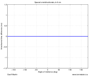
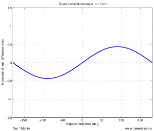
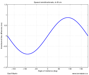
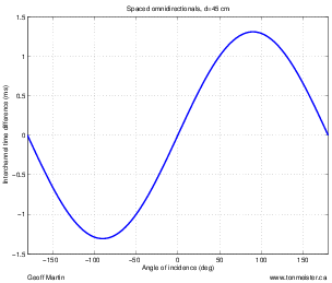
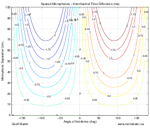
One of the big problems with looking at microphone polar responses in only the horizontal plane is that we usually don’t only have sound sources restricted to those two dimensions. Invariably, we tend to raise or lower the microphone stand to obtain a different direct-reverberant ratio, for example, without considering that we’re also changing the vertical angle of incidence to the microphone pair. In almost all cases, this has significant effects on the response of the pair which can be seen in a three-dimensional anaysis.
In order to include vertical angles in our calculations of microphone sensitivity, we need to use a little spherical trigonometry – not to worry though. The easiest way to do this is to follow the instructions below:
The answer to this last question is actually pretty easy. If we call the horizontal angle of rotation ϑ, matching the angle in the horizontal plane we talked about earlier, and the vertical angle of rotation ϕ, then the total resulting angle γ can be calulated using Equation 10.6.
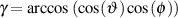 | (10.6) |
Now, there’s one nice little thing about this equation. Since we’re talking about microphone sensitivity patterns, and since the only part of this pattern is dependent on the Pressure Gradient component of the microphone, and since this component only relies on the cosine of the angle of incidence, then we don’t need to do as much math. For example, what we’re really interested in is cos(γ) but we can only calculate γ by doing an arccos function. So, instead of using Equation 10.6, we can simplify it to Equation 10.8.
There’s one more thing. In order to simplify our lives a bit, I’m going to restrict the included angle between the microphones to the horizontal plane. Basically, this means that, for all three dimensional analyses in this paper, we’re thinking that we have a pair of microphones that’s set up parallel to the floor, and that the instrument can be at any angle of incidence to the pair. That angle of incidence is comprised of an angle of rotation and an angle of elevation. We’re not going to have the luxury of tilting the microphone pair on its side (unless you’re able to just think of that as moving the instrument to a new position...).
So, in order to convert Equation 10.3 into a three-dimensional version, we combine it with Equation 10.8, resulting in Equation 10.9.
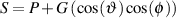 | (10.9) |
This can include the horizontal rotation of the microphone, Ω as follows:
 | (10.10) |
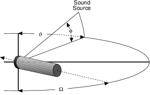
3-D Polar Coordinate Systems
Some discussion should be made here regarding the issue of different three-dimensional polar coordinate systems. Microphone polar patterns in three dimensions are typically described using the spherical coordinate system which uses two angles referenced to the origin on the surface of the sphere at the location (0, 0). The first, α, is an angle of rotation in the horizontal axis around the centre of the sphere. The second, δ, is an angle of rotation around the axis intersecting the centre of the sphere and the origin. This is shown on the right in Figure 10.77. In the case of microphones, the origin is thought of as being located at the centre of the diaphragm of the microphone and the axis for the rotation δ is perpendicular to the diaphragm.
The geographic coordinate system also uses two angles of rotation. Similar to the spherical coordinate system, the first, ϑ, is a rotation around the centre of a sphere in the horizontal plane from the origin at the location (0,0). In geographic terms, this would be the measurement of longitude around the equator. The second angle, ϕ, is slightly different in that it is an orthogonal rotation off the equator, also rotating around the sphere’s centre. The geographic equivalent of this vertical rotation is the latitude of a location as can be seen on the left in Figure 10.77.
This investigation uses the geographic coordinate system for its evaluation in order to make the explanations and figures more intuitive. For example, when a recording engineer places a microphone pair in front of an ensemble and raises the microphone stand, the resulting change in polar location of the instruments relative to the array is a change in elevation in the geographic coordinate system. These changes in the angle of elevation of the microphone pair can correspond to changes in ϕ up to ±90∘.
One issue to note in the use of the geographic coordinate system is the location of positions with values of ϕ outside the ±90∘ window. It must be kept in mind that these positions produce and alternation from left to right and vice versa. Therefore ϑ = 45∘,ϕ = 180∘ is in the same location as ϑ = -135∘,ϕ = 0∘
Although the use of the geographic coordinate system makes the figures and discussion of microphone pair characteristics more intuitive, this unfortunately comes at the expense of a somewhat increased level of complexity in the calculations.
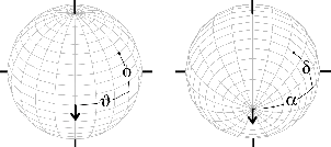
Cardioids
We’ll begin with a pair of coincident cardioid microphones. Figures 10.78 and 10.79 show plots of the interchannel amplitude difference of a pair of cardioids with an included angle of 90∘. (Unfortunately, if you’re looking at a black and white printout of this paper, you’re going to have a bit of a problem seeing things... sorry...)
Take a look at the spherical plot in Figure 10.78. If we look at the value in dB plotted on this sphere around its equator, we’d get exactly the same graph as is shown in Figure 10.49. Now, however, we can see that changes in the vertical angle might have an effect on the way things sound. For example, if we have a sound source with a vertical elevation of 0∘ and a horizontal rotation of 90∘, then the interchannel amplitude difference is about 18 dB, give or take (to get this number, I cheated and looked back at Figure 10.50). Now, if we maintain that angle of rotation and change the vertical angle, we reduce this difference until, with a vertical angle of 90∘, the interchannel amplitude difference is 0 dB – in other words, if the sound source is directly above the pair, the outputs of the two mic’s are the same.
What effect does this have on our phantom image location in the real world? Let’s go do a live-to-two-track recording where we set up a 90∘ pair of cardioids at eye level in front of an orchestra at the conductor’s position. This means that your principal double bass player is at a vertical angle of 0∘ and a horizontal angle of 90∘, so that instrument will be about 18 dB louder in the right channel than in the left. This means that its phantom image will probably be parked in the right speaker. We start to listen to the sound and we decide that we’re too close to the orchestra – and since we read a rule from an unreliable source that concert halls always sound much better if you go up about 4 or 5 m, we’ll raise the mic stand way up. This means that the double bass is still at an angle of rotation of 90∘, but now at a vertical angle of about 60∘ (we went really high). This means that the interchannel amplitude difference for the instrument has dropped to about 6 dB, which would put it well inside the right loudspeaker in the recording.
So, the moral of the story is, if you have a pair of coincident cardioids and you raise your mic stand without pointing the mic’s downwards to compensate, your orchestra gets narrower in the stereo image. Also, don’t forget that this doesn’t just apply to two-channel stuff. We could just as easily be talking about the image between your surround loudspeakers.
Figure 10.79 shows a contour map of the same plot shown in Figure 10.78 which makes it a little easier to read. Now, the two angles are the X- and Y-axes of the graph, and the lines indicate the angles where a given interchannel amplitude difference occurs. From this, you can see that, unless your rotation is 0∘, then any change in the vertical angle, upwards or downwards, will reduce your interchannel difference. This is true for all included angles (except for 0∘) of a pair of coincident cardioids.
There’s one more thing to consider here, and that the fact that the microphones are not just recording an instrument – they’re recording the room as well. So, you have to keep in mind that, in the case of coincident cardioids, all reflections and reveberation that come from above or below the microphones will tend to pull towards the centre of your loudspeaker pair. Again, the greater the angle of elevation, the more the image collapses.
Subcardioids
Subcardioids have a pretty predictable behaviour, now that we’ve looked at the response patterns of cardioid microphones. The only big difference is that, as we’re seen before, the interchannel amplitude difference never goes outside the ±6 dB window. Apart from that, the responses are not too different.
Bidirectionals
Now, let’s compare those results with a pair of coincident bidirectional microphones instead. One caveat here before we begin, because we’re looking at decibel scales, and because calculators don’t like being asked to find the logarithm of a negative number, we’re looking at the absolute value of the sensitivity of the microphones again.
This time, the plots tell a very different story. Notice how, in the spherical plot in Figure 10.88 and in the contour plots in Figures 10.89 through 10.91, we get a bunch of vertical lines. The summary of what that means is that the interchannel amplitude difference of a pair of bidirectional microphones doesn’t change with changes in the angle of elevation. So you can raise and lower the mic stand all you want without collapsing the image of the orchestra. As we get further off axis (because we’ve changed the vertical angle), the orchestra will get quieter, but it won’t pull to the centre of the loudspeakers. This is a good thing.
There is a small drawback here, though. Remember that if you have a big vertical angle, then a small horizontal movement of the instrument corresponds to a large change in the angle of rotation, so you can get a violent swing in the image location if you’re not careful. For example, if your bidirectional pair is really high and you’re recording a singer that likes to sway back and forth, you might wind up with a phantom image that is always swinging back and forth between the two speakers, making your listeners seasick.
Also, note with a pair of bidirectional microphones with an included angle of 180 degrees that all angles of incidence produce the same sensitivity – just remember that the two signals are of opposite polarity. If you want to do this, use your “phase flip” button. It’s cheaper than a second microphone.
Hypercardioids
Once again, hypercardioids exhibit properties that are recognizable as being something between a cardioid and a bidirectional. If we look at the spherical plot of a pair of coincident hypercardioids with an included angle of 90∘ shown in Figure 10.93, we can see that there is a dividing line along the side of the pair, similar to that found in a bidirectional pair. Just like the bidirectionals, this follows the null point in one of the two microphones, the dividing line between the front and rear lobes. However, like the cardioid pair, notice that vertical changes alter the interchannel amplitude difference. There is one big difference from the cardioids, however. In the case of cardioids, a vertical change always results in a reduction in the interchannel amplitude difference whereas, in the case of a hypercardioid pair, it is possible to have a vertical change that produces an increase in the interchannel amplitude difference. This is most easily visible in the contour plot in Figure 10.95. Notice that if you start with a horizontal angle of 100 degrees, then a vertical change off the equator will cause the interchannel amplitude difference to increase to ∞ dB before it reduces back down to 0 dB at the north or south pole.
There are three principal practical issues to consider here. Firstly, remember that a change in the height of your mic stand with a pair of hypercardioids will change the apparent width of your sound stage. Unlike the case of cardioids, however, the change might wind up increasing the width of some components while simultaneously decreasing the width of others. So you wind up squeezing together the centre part of the orchestra while you pull apart the sides.
The second issue to consider is similar to that with cardioids. Don’t forget that you’ve got sound coming in from all angles at the same time - so it’s possible that some parts of your room sound will be pulled wider while others are pushed closer together.
Thirdly, there’s just the now-repetitious reminder that a lot of the signals coming into the pair are arriving at the rear lobes of the microphones, so you’re going to have signals that are either in opposite polarity in the two channels, or similar, but inverted polarities.
Spaced omnidirectionals
Calculation of the interchannel time of arrival differences for a pair of spaced microphones in a three-dimensional world requires only a small change to Equation 10.4 as can be seen in Equation 10.11.
 | (10.11) |
Consider that a change in elevation in the geographic coordinate system means that we are heading away from the “equator” towards the “north pole”, relative to the microphones. When the sound source is located at any angle of horizontal rotation and an angle of elevation ϕ = 90∘, it is equidistant from the two microphones, therefore the time of arrival difference is 0 ms. Consequently, we can intuitively see that the greatest time of arrival difference is for sources where ϕ = 0∘, and that any change in elevation away from this plane will result in a reduced value of ΔTime.
This behaviour can be seen in Figures 10.98 through 10.100 as well as Figure 10.101.
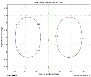
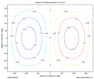
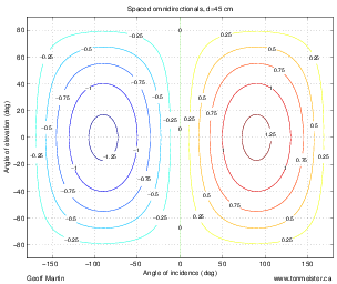
The previous chapter deals only with the interchannel differences between the two microphones in a pair. This information gives us an idea of the general placement of phantom images between pairs of loudspeakers in a playback system, but there are a number of other issues to consider. Back in the discussion on panning in Chapter 10.3.1, something was mentioned that has not yet been discussed. As was pointed out, pan knobs on consoles work by changing the amplitude difference between the output channels, but the issue of why they are typically constant power panners was not mentioned.
Since we’ve been thinking of microphone pairs as panning algorithms, we’ll continue to do so, but this time looking at the summed power output of the pair. Since the power of a signal is proportional to the square of its amplitude, this can be done using Equation 10.12.
 | (10.12) |
where O is the total output power of the two microphones.
In order to calculate this power response curve on a decibel scale, the following equation is used:
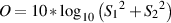 | (10.13) |
The question, of course, is “What will this tell us?” I’ll answer that question using the example of a pair of coincident cardioid microphones.
Cardioids
Figure 10.102 shows the summed power response of a pair of coincident cardioid microphones with an included angle of 90∘. as you can see, the total power for sources with an angle of incidence of 0∘ is about 2 dB. As you rotate away from the front of the pair, the summed power drops to a minimum of about -12 dB directly behind. Remember from the previous chapter that the 0∘ and 180∘ locations in the horizontal plane are the two positions where the interchannel amplitude difference is 0 dB, therefore instruments in these two locations will result in phantom images between the two loudspeakers, however, we can now see that, although this is true, the two images will differ in power by approximately 15 dB, with sources in the front of the microphone pair being louder than those behind.
The range of the summed power for a pair of cardioids changes with the included angle as is shown in Figures 10.102 through 10.105. In fact, the smaller the included angle, the greater the range. As can be seen in Figure 10.103, the range of summed power is approximately 28 dB compared to only 3 dB for an included angle of 180∘. Also note that for larger included angles, there are two symmetrical peaks in the power response rather than one at an angle of incidence of 0∘.
Each of these analyses, in conjunction with their corresponding interchannel amplitude difference plot for the same included angle, gives us an indication of the general distribution of energy across the reproduced sound stage. For example, if we look at a pair of coincident cardioids with an included angle of 45∘, we can see that instruments, reflections and reverberation with an angle of incidence of 0∘ are much louder than those away from the front of the pair. In addition, we can see from the ΔAmp. plot that a large portion of sources around the pair will image near the centre position between the loudspeakers. Consequently, the resulting sound stage appears to “clump” in the middle rather than being spread evenly across the playback room.
In addition, for smaller included angles, it can be seen that much more emphasis is placed on sound sources and reflections in the front of the pair with sources to the rear attenutated.
Subcardioids
Figures 10.106 through 10.109 show the summed power plots for the horizontal plane of a pair of subcardioid microphones. As is evident, there is a much smaller range of values than is seen in the cardioid microphones, however the general shape of the curves are similar. As can be seen in these plots, there is a more evenly distributed sensitivity to sound sources and reflections around the microphone pair, however, due to the limited range of values for ΔAmp., these sources typically image between the loudspeakers as well.
Bidirectionals
Due to the symmetrical double lobes of bidirectional microphones, they exhibit a considerably different power response as can be seen in Figures 10.110 through 10.113. When the included angle of the microphones is 90∘, there is a constant summed power throughout all angles of incidence. Consequently, all sources around the pair apper to have the same level at the listening position, regardless of angle of incdence. If the included angle of the pair is reduced as is shown in Figure 10.110, then we reduce the apparent level of sources to the side of the microphone pair. When the included angle is greater than 90∘, the dips in the power response happen directly in front of and behind the microphone pair.
Notice as well that bidirectional pairs differ from cardioids in that the high and low points in the summed power response are always in the same locations – 0∘, 90∘, 180∘ and 270∘. They do not move with changes in included angle, they simply change power level.
Note now that we are not talking about the absolute value of the sensitivity of the microphones. This is because the calculation of power automatically squares the sensitivity, thus making all values postive and therefore making the logarithm happy...
Hypercardioids
Once again, hypercardioids behave like a hybrid between cardioids and bidirectionals as can be seen in Figures 10.114 through 10.117.
Spaced omnidirectionals
It is typically assumed that the outputs levels of omnidirectional microphones are identical, differing only in time of arrival. This assumption is incorrect for sources whose distance to the pair is similar to the distance between the mic’s, or when you’re using omnidirectionals that aren’t really omnidirectional. Both cases happen frequently, but we’ll stick with the assumption for this paper. As a result, we’ll assume that the summed power output for a pair of omnidirectional microphones is +3 dB relative to either of the microphones for all angles of rotation and elevation.
As before, we can only get a complete picture of the response of the microphones by looking at a three-dimensional response plot.
Cardioids
The three dimensional plots for cardioids hold no surprises. As we can see, for smaller included angles as is shown in Figure 10.119, the range of values for the summed power is quite wide, with the high and low points being at the front and rear of the pair respectively, on the “equator.”
If the included angle is increased beyond 90∘, then two high points in the power response appear on either side of the front of the pair. Meanwhile, as was seen in the two-dimensional analyses, the overall range is reduced with a smaller attenuation behind the pair.
Subcardioids
Again, subcardioid microphones behave similar to cardioids with a smaller range in their summed power response.
Bidirectionals
Bidirectional microphone pairs have a rather interesting property at 90∘. Note in Figure 10.129 that the contour plot for the summed power for the microphone pair shows a number of horizontal lines. This means that if you have a sound source at a given angle of elevation, changes in the angle of rotation will have no effect on the apparent level of the sound source. This, in turn, means that all sources at a given angle of elevation have the same apparent total gain.
Additionally, notice that the point where the total power is the greatest is the horizontal plane, with a value of 0 dB with decreasing level as we move away from the equator.
As was seen in the two-dimensional plots, included angles of less than 90∘ cause the high points in the power plots to occur at the front and rear of the pairs as is shown in Figure 10.130. Notice that, unlike the cardioid and subcardioid pairs, the minimum points (with a value of -∞ dB) are directly above and below the microphone pair. This is true for bidirectional pairs with any included angle.
As can be seen in Figures 10.131 and 10.132, when the included angle is greater than 90∘, the behavour of the pair is exactly the same as the symmetrical included angle less than 90∘, with a 90∘ rotation in the behavour. For example, pairs with included angles of 70∘ and 110∘ (symmetrical around 90∘) have identical responses, but where the 70∘ pair is “pointing” forward, the 110∘ pair is “pointing” sideways.
Hypercardioids
Finally, as we have seen before, the hypercardioid pairs exhibit a response pattern that is a combination of the cardioid and bidirectional patterns. One important thing to note here is that, although the location with the highest summed power value is on the horizontal plane as in the case of the cardioid microphones, the point of minimum power is between the equator and the poles in all cases but an included angle of 180∘.
Finally, we’ll take a rather holistic view of the pair of microphones and take a look at the correlation coefficient and coherence of their outputs. This can give us a general idea of the similarity of the two signals which could be interpreted as a sensation of spaciousness, but will also give us an indication of how much we have to worry about interference between channels. We have to be very careful here in making this jump between correlation, coherence and spaciousness as will be discussed below, but first, we’ll look at exactly what is meant by the terms “correlation” and “coherence.”
If you’re not absolute certain what is mean by the term correlation coefficient you should read Section 4.14.
If you’re not absolute certain what is mean by the term coherence you should read Section 9.6.5.
In the field of perception of concert hall acoustics, it has long been known that there is a link between Interaural Cross Correlation (IACC) and a perceived sensation of diffuseness and auditory source width (ASW)[Ando, 1998]. (IACC is a measure of the cross-correlation between the signals at your two ears.) The closer the IACC approaches 1, the lower the subjective impression of diffuseness and ASW. The lower the IACC, the more diffuse and wider the perceived sound field.
One of the nice things about recording is that you can control the IACC at the listening position by controlling the interchannel correlation coefficient. Although the interchannel correlation coefficient doesn’t directly correspond to the IACC, they are related. In order to figure out the exact relationship bewteen these two measurements, you’ll also need to know a little bit about the room that the speakers are in.
There are a couple of things to remember about interchannel correlation that we have to remember before we start talking about microphone response characteristics.
A free-field situation is one where the waveform is free to expand outwards forever. This typically only happens in thought experiments, however we typically assume that the situation exists in anechoic chambers and on the top of poles outdoors. To extend our assumptions even further, we can simplify the direct sound from a sound source received at a microphone to be considered as a free field source. Consequently, the analysis of a microphone pair in a free field becomes applicable to real life.
Coincident pairs
If we convert Equation 4.1 to something that represents the signal at the two microphones, then we wind up with Equation 10.14 below.
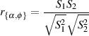 | (10.14) |
where r is the correlation coefficient of the outputs of the two microphones with sensitivities S1 and S2 for the angles of rotation α and elevation ϕ.
Luckily, this can be simplified to Equation 10.15.
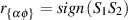 | (10.15) |
where the function sign(x) indicates the polarity of x. sign(x) = 1 for all x > 0, sign(x) = -1 for all x < 0 and sign(x) = 0 for all x = 0
This means that, for coincident omnidirectional, subcardioid and cardioid microphones, all free field sources have a correlation of 1 all the time. This is because the only theoretical difference between the outputs of the two microphones is in their level. The only exception here is the particular case of a sound source located exactly at the null point for one of the cardioids in a pair. In this location, the correlation coefficient of the two outputs will be 0 because one of the channels contains no signal.
In the case of hypercardioids and bidirectionals, the value of the correlation coefficient for variou free field sources will be either 1, 0 or -1. In locations where the polarities of the two signals are the same, either both positive or both negative, then the correlation coefficient will be 1. Sources located at the null point of at least one of the microphones will produce a correlation coefficient of 0. Sources located in positions where the receiving lobes have opposite polarities (for example, to the side of a Blumlein pair of bidirectionals), the correlation coefficient will be -1.
Spaced omnidirectionals
As was discussed above, spaced omnidirectional microphones are used under the (usually incorrect) assumption that the only difference between the two microphones in a free field situation will be their time of arrival. As was shown in Figure 10.70, this time separation is dependent on the spatial separation of the two microphones and the angles of rotation and elevation of the source to the pair.
The result of this time of arrival difference caused by the extra propagation distance is a frequency-dependent phase difference between the two channels. This interchannel phase difference ωτ can be calculated for a given additional propagation distance using Equation 10.16.
 | (10.16) |
where λ is the acoustic wavelength in air.
This can be further adapted to the issue of microphone separation and angle of incidence by combining Equations 10.4 and 10.16, resulting in Equation 10.17.
 | (10.17) |
where ωτ{ϑ,ϕ} is the frequency-dependent phase difference between the channels for a sound source at angle of rotation ϑ, angle of elevation ϕ, and k is the acoustic wavenumber, defined in Equation 10.18 [Morfey, 2001].
 | (10.18) |
where c is the speed of sound in air.
Consequently, we can calculate the correlation coefficient for the outputs of two omnidirectional microphones with a free field source using the model of a single signal correlated with a delayed version of itself. This is calculated using Equation 10.19.
 | (10.19) |
All we need to do is to insert the phase difference of the two microphones, calculated using Equation 10.17 into this equation and we’ll see that the correlation coefficient is a complete mess.
So now the question is “do we care?” The answer is “probably not.” Why not? Well, the correlation coefficient in this case is dependent on the phase relationship between the two signals. Typically, if you present a signal to a pair of loudspeakers where the only difference is their time of arrival at the listening position, then you probably aren’t paying attention to their phase difference – it’s more likely that you’re more interested in their time difference. This is because the interaural time of arrival difference is such a strong cue for localization of sources in the real world. Even for something we’d consider to be a “steady state” source like a melodic instrument playing slow music, the brain is grabbing each little cue it can to determine the time relationship. The only time the interchannel phase information (and therefore the free field correlation coefficient) is going to be the predominant cue is if you listen to sinusoidal waves – and nobody wants to do that...
Now we have to talk about what a diffuse field is. If we get into the official definition of a diffuse field, then we have to have a talk about things like infinity, plane waves, phase relationships and probability distribution... maybe some other time... Instead, let’s think about a diffuse field in a couple of different, equally acceptable ways. One way is to think that you have sound coming from everywhere simultaneously. Another way is that you have sound coming from different directions in succession with no time inbetween their arrival.
If we think of reverberation as a very, very big number of reflections coming from all directions in fast succession, then we can start to think of what a diffuse field is like. Typically, we like to think of reveberation as a diffuse field – this is particularly true for the people that make digital reverb units because it’s much easier to create random messes that sort of sound like reverb than it is to calculate everything that happens to sound as it bounces around a room for a couple of seconds.
We need to pay a lot of attention to the correlation coefficient of the diffuse component of the recorded signal. This can be used as a rough guide to the overall sense of “spaciousness” (or whatever word you wish to use – this area creates a lot of discussion) in your recording. If you have a correlation coefficient of 1, this will probably mean that you have a reverberant sound that is completely clumped into one location between the two loudspeakers. The only possible exception to this is if your signals are going to the adjacent pair of front and surround loudspeakers (i.e. Left and Left Surround) where you’ll find it very difficult to obtain a single phantom location.
If your correlation coefficient is -1, then you have what most people call two “out of phase” signals, but what they really are is identical signals with opposite polarity.
If your correlation coefficient is 0, then there could be a number of different explanations behind the result. For example, a pair of coincident bidirectionals with an included angle of 90∘ will have a correlation coefficient of 0. If we broke the signals hitting the two diaphragms into individual sounds from an infinite number of sources, then each one would have a correlation coefficient of either 1 or -1, but since there are as many 1’s as -1’s, the whole diffuse field averages out to a total correlation of 0. Although the two signals appear to be completely uncorrelated according to the math, there will be an even distribution of sound between the speakers (because there are some components in there that have a correlation of 1, remember...)
On the other hand, if we take two omnidirectional microphones and put them very, very far apart – let’s put them in completely different rooms to start, then the two signals are completely unrelated, therefore the correlation coefficient will be 0 and you’ll get an image with no phantom sources at all – just two loudspeakers producing a pocket of sound. The same is true if you place the omni’s very far apart in the same concert hall (you’ll sometimes see engineers doing this for their ambience microphones). The resulting correlation coefficient, as we’ll see below, will also be 0 because the sound fields at the two locations will sound similar, but they’ll be completely unrelated. The result is a hall with a very large hole in the middle – because there are no correlated components in the two signals, there cannot be an even spread of energy between the loudspeakers.
The moral of the story here is that, in order to keep a “spacious” sound for your reverb, you have to keep your correlation coefficient close or equal to 0, but you can’t just rely on that one number to tell you everything. Spacious isn’t necessarily pretty, or believable...
Coincident pairs
Calculating the correlation of the outputs of a pair of coincident microphones is somewhat less than simple. In fact, at the moment, I have to confess that I really don’t know the correct equation for doing this. I’ve searched for this piece of information in all of my books, and I’ve asked everyone that I think would know the answer, and I haven’t found it yet. So, I wrote some MATLAB code to model the situation instead of doing the math the right way. In other words, I did a numerical calculation to produce the plots in Figures 10.138 and 10.139, but this should give us the right answer.
Some of the characteristics see in Figure 10.138 should be intuitive. For example, if you have a pair of coincident omnidirectional microphones in a diffuse field, then the correlation coefficient of their outputs will be 1 regardless of their included angle. This is because the outputs of the two mic’s will be identical no matter what the angle.
Also, if you have any matched pair of microphones with an included angle of 0∘, then their outputs will also be identical and the correlation coefficient will be 1.
Finally, if you have a pair of matched bidirectional microphones with an included angle of 180∘, then their outputs will be identical but opposite in polarity, therefore their correlation coefficient will be -1.
Everything else on that plot will be less obvious.
Just in case you’re wondering, here’s how I calculated the two graphs in Figures 10.138 and 10.139.
If you have a pair of coincident bidirectional microphones with an included angle of 90∘ in a diffuse field, then the correlation coefficient of their outputs will be 0. This is somewhat intuitive if we think that half of the field entering the microphone pair will have a correlation of 1 (all of the sound coming from the front and rear of the pair where the lobes have matched polarities) while the other half of the sound field results in a correlation of -1 (because it’s entering the sides of the pair where you have opposite polarity lobes.) Since the area producing the correlation of 1 is identical to the area producing the correlation of -1, then the two cancel each other out and produce a correlation of 0 for the whole.
Similarly, if we have a coincident bidirectional and an omnidirectional in a diffuse field, then the correlation coefficient of their outputs will also be 0 for the same reason.
As we’ll see in Section 10.5, if you have a coincident trio of microphones consisting of two bidirectionals at 90∘ and an omni, then you can create a microphone pointing in any direction in the horizontal plane with any polar pattern you wish – you just need to know what the relative mix of the three mic’s should be.
Using MATLAB, I produced three uncorrelated vectors containing a bunch of 10000 random numbers, each vector representing the output of each of the three microphones in that magic array described in the previous paragraph sitting in a noisy diffuse field. I then made two mixes of the three vectors to produce a simulation of a given pair of microphones. I then simply asked MATLAB to give me the correlation coefficient of these two simulated outputs.
If someone could give me the appropriate equation to do this the right way, I would be very grateful.
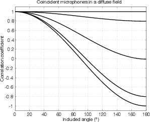
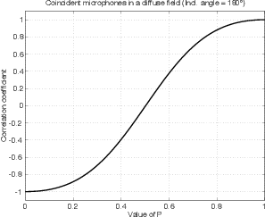
Spaced omnidirectionals
If we have a pair of omnidirectionals spaced apart in a diffuse field, then we can intuitively get an idea of what their correlation coefficient will be. At 0 Hz, the pressure at the two locations of the microphones will be the same. This is because the sound pressure variations in the room are all varying the day’s barometric pressure which is, for our purposes, 0 Hz. At very low frequencies, the wavelengths of the sound waves going past the microphones will be longer than the distance between the mic’s. As a result, the two signals will be very correlated because the phase difference between the mic’s is small. As we go higher and higher in frequency, then the correlation should be less and less, until, at some high frequency, the wavelengths are much smaller than the microphone separation. This means that the two signals will be completely unrelated and the correlation coefficient goes to 0.
In fact, the relationship is a little more complicated than that, but not much. According to Kutruff [Kutruff, 1991], the correlation coefficient of two spaced locations in a theoretical diffuse field can be calculated using Equation 10.20.
 | (10.20) |
where k is the “wave number.” This is a slightly different way of saying “frequency” as can be seen in Equation 10.21 below (also see Equation 10.18).
 | (10.21) |
Note that k is proportional to frequency and therefore inversely proporational to wavelength.
If we were to calculate the correlation coefficient for a given microphone separation and all frequencies, the plot would look like Figure 10.140. Note that changes in the distance between the mic’s will only change the frequency scale of the plot – the closer the mic’s are to each other, the higher the frequency range of the area of high correlation.
Also known as Mid-Side or Mono-Stereo
We have already seen that any microphone polar pattern can be created by mixing an omnidirectional with a bidirectional microphone. Let’s look at what happens when we mix other polar patterns.
We’ll begin with a fairly simple case – two bidirectional microphones, one facing forward towards the middle of the stage (the “mid” microphone) and the other facing to the right (the “side” microphone). If we plot these two individual polar patterns on a cartesian plot the result will look like Figure 10.141.
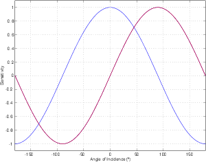
The same can be shown as the more familiar polar plot, displayed in Figure 10.142.
Now, let’s take those two microphone outputs and, instead of sending them to the left and right outputs as we normally do with stereo microphone configurations, we’ll send them both to the right output by panning both channels to the right. We’ll also drop their two levels by 3 dB while we’re at it (we’ll see why later...)
What will be the result? We can figure this out mathematically as is shown in the equation below.
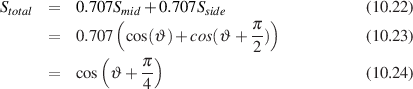
If we were to plot this, it would look like Figure 10.143.
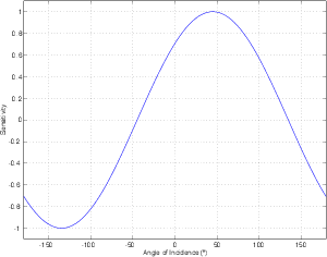
You will notice that the result is a bidirectional microphone aimed 45∘ to the right. This shouldn’t really come as a big surprise, based on the assumption that you’ve read Section 1.5 way back at the beginning of this book.
In fact, using the two bidirectional microphones arranged as shown in Figure 10.141, you can create a “virtual” bidirectional microphone facing in any direction, simply by adding the outputs of the two microphones with carefully-chosen gains calculated using Equations 10.25 and 10.26.
 | (10.25) |
 | (10.26) |
where M is the gain applied to the mid bidirectional, S is the gain applied to the side bidirectional and σ is the desired on-axis angle of the virtual bidirectional.
One important thing to notice here is that, for some desired angles of the virtual bidirectional microphone, you’re going to have a negative gain on at least one of your microphones – possibly both of them. This, however, is easy to accomplish on your average mixing console. You just have to hit the polarity flip switch.
So, now we’ve seen that, using only two bidirectional microphones and a little math, you can create a bidirectional microphone aimed in any direction. This might be particularly useful if you don’t have time to do a sound check before you have to do a recording (yes... it does happen occasionally). If you set up a pair of bidirectionals, one mid and one side and record their outputs straight to a two-track, you can do the appropriate summing later with different gains for your two stereo outputs to create a virtual pair of bidirectional microphones with an included angle that is completely adjustable in post-production. The other beautiful thing about this technique is that, if you are using bidirectional microphones whose front and back lobes are matched to each other on each microphone, your resulting matrixed (summed) outputs will be a perfectly matched pair of bidirectionals – even if your two original microphones are not matched... they don’t even have to be the same brand name or model... Let’s say that you really like a Beyer M130 ribbon microphone for its timbre, but the SNR is too low to use to pick up the sidewall reflections, you can use it for the mid, and something like a Sennheiser MKH30 for the side bidirectional. Once they’re matrixed, your resulting virtual pair of microphones (assuming that you have symmetrical gains on your two outputs) will be perfectly matched. Cool huh?
You are not restricted to using two similar polar patterns when you use matrixing in your microphone techniques. For example, most people when they think of MS, think of a cardioid microphone for the mid and a bidirectional for the side. These two are shown in Figures 10.144 and 10.145.
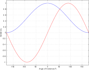
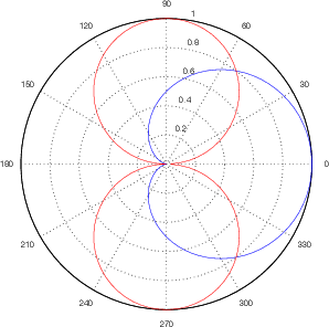
What happens when we mix the outputs of these two microphones? Well, in order to maintain a constant on-axis response for the virtual microphone that results, we know that we’re going to have to attenuate the outputs of the real microphones before mixing them. So, let’s look at an example of the cardioid reduced by 6.02 dB and the bidirectional reduced by 3.01 dB (we’ll see why I chose these particular values later). If we were to express the sensitivity of the resulting virtual mic as an equation it would look like Equation 10.27
 | (10.27) |
What does all this mean? Svirtual is the sensitivity of the virtual microphoneThe first
0.5 is there because we’re dropping the level of the cardioid by 6 dB, similarly the 0.707
is there to drop the output of the bidirectional by 3 dB. The output of the cardioid should
be recognizable as the 0.5+0.5cos(ϑ). The bidirectional is the part that says
cos(ϑ - ). Note that the
  is there because we’ve turned the bidirectional 90∘.
(An easier way to say this is to use sin(ϑ) instead – it will give you the same
results.
is there because we’ve turned the bidirectional 90∘.
(An easier way to say this is to use sin(ϑ) instead – it will give you the same
results.
If we graph the result of Equation 10.27 it will look like Figure 10.146. Note that the result is a traditional hypercardioid pattern “aimed” at 71∘.
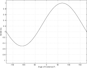
There is a common misconception that using a cardioid and a bidirectional as an MS pair will give you a pair of virtual cardioids with a controllable included angle. This is not the case. The polar pattern of the virtual microphones will change with the included angle. This can be seen in Figure 10.147 which shows 10 different balances between the cardioid mid microphone and the bidirectional side.
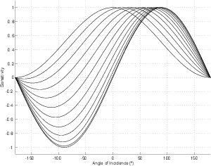
How do you know what the relative levels of the two microphones should be? Let’s look at the theory and then the practice.
Theory
If you wanted to maintain a constant on-axis sensitivity for the virtual microphone as it rotates, then we could choose an arbitrary number n and do the math in Equations 10.28 and 10.29:
 | (10.28) |
 | (10.29) |
This M and S are the gains to be applied to the cardioid and bidirectional feeds, respectively. If you were to graph this relationship it would look like Figure 10.148.
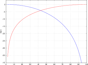
You’ll notice that I haven’t spent much time on this theoretical side. This is because it has so little to do with the practical usage of MS mic’ing. If you wanted to really do this the right way, then I’d suggest that you do things a slightly different way. Use the math in Section 10.5.1 to create a virtual bidirectional pointing in the desired direction, then add some omni to produce the desired polar pattern. This idea will be elaborated in Section 10.5.2.
Practice
Okay, if you go to do an MS recording, I’ll bet money that you don’t bring your calculator along to do any of the math I just described. Use the following steps...
Don’t feel obliged to keep your two bidirectional gains equal. Just remember that if they’re not, then the polar patterns of your two virtual microphones are not matched. Also, they will not be aimed symmetrically, but that might be a good thing... People listening to the recording at home won’t know whether you used a matched pair of microphones or not.
To a large portion of the population who have encountered the term, “Ambisonics” generally means one of two things :
In actual fact, is really neither of these things. Ambisonics is more of a mathematical concept and technique which is an attempt to reproduce a recorded soundfield. This idea differs from most stereo and surround recordings in that the intention is to re-create the acoustic wavefronts which existed in the space at the time of the recording rather than to synthesize an interpretation of an acoustic event.
Go to a room (you may already be in one...) and put a perfect omnidirectional microphone in it. As we discussed in Section 6.7, an omnidirectional microphone is also known as a pressure transducer which means that it responds to the changes in air pressure at the diaphragm of the microphone. If you make a perfect recording of the output of the perfect omnidirectional microphone when stuff is happening in the room, you have captured a record (here, I’m using the word “record” as in a historical record, not as in a record that you buy at a record shop from a record lady[Lovett, 1994]) of the change in pressure over time at that location in that room on that day. If, at a later date, you play back that perfect recording over a perfect loudspeaker in a perfectly anechoic space, then you will hear a perfect representation (think “re-presentation”) of that historical record. Interestingly, if you have a perfect loudspeaker and you’re in a perfectly anechoic space, then what you hear from the playback is exactly what the microphone “heard” when you did the recording.
This is a good idea, however, let’s take it a step farther. Since a pressure transducer has an omnidirectional polar pattern, we don’t have any information regarding the direction of travel of the sound wavefront. This information is contained in the velocity of the pressure wave (which is why a single directional microphone of any sort must have a velocity component). So, let’s put up a perfect velocity microphone in the same place as our perfect pressure microphone. As we saw in Section 6.7 a velocity microphone (if we’re talking about directional characteristics and not transducer design) is a bidirectional microphone. Great, so we put a bidirectional mic facing forward so we can tell if the wave is coming from the front or the rear. If the outputs of the omni and the bidirectional have the same polarity, then the sound source is in the front. If they’re opposite polarity, then the sound source is in the rear. Also, we can see from the relative levels of the two mic outputs what the angle to the sound source is, because we know the relative sensitivities of the two microphones. For example, if the level is 3 dB lower in the bidirectional than the omni and both have the same polarity, then the sound source must be 45∘ away from directly forward. The problem is that we don’t know if it’s to the left or the right. This problem is easily solved by putting in another bidirectional microphone facing to the side. Now we can tell, using the relative polarities and outputs of the three microphones where the sound source is... but we can’t tell what the sound source elevation is. Again, no problem, we’ll just put in a bidirectional facing upwards.
So, with a single omni and three bidirectionals facing forward, to the right and upwards, we can derive all sorts of information about the location of the sound source. If all four microphones have the same polarity, and the outputs of the three bidirectionals are each 3 dB below the output of the omni, then the sound source must be 45∘ to the right and 45∘ up from the microphone array.
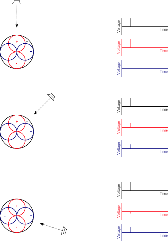
Take a look at the top example in Figure 10.149. We can see here that if the sound source is directly in front of the microphone array, then we get equal positive outputs from the omni (we’ll call this the W channel) and the forward-facing bidirectional (we’ll call that one the Y channel) and nothing from the side-facing bidirectional (the X channel). Also, if I had been keen and did a 3D diagram and drawn the upwards-facing bidirectional (the Z channel), we’d see that there was no signal from that one either if the sound source is on the same horizontal plane as the microphones.
Let’s record the pressure wave (using the omni mic) and the velocity, and therefore the directional information (using the three bidirectional mic’s) on a perfect four-channel recorder. Can we play these channels back to reproduce all of that information in our anechoic listening room? Take a look at Figure 10.150.
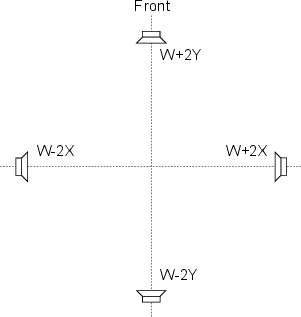
Let’s think about what happens to the sound source in the top example in Figure 10.149 if we play back the W, X, and Y channels through the system in Figure 10.150. In this system, we have four identical loudspeakers placed at 0∘, 180∘, and ±90∘. These loudspeakers are all identical distances from the sweet spot.
The top example in Figure 10.149 results in a positive spike in both the W and Y channels, and nothing in the X channel. As a result, in the playback system:
The loudspeakers produce a signal at exactly the same time, and the different waves will propagate towards the sweet spot at the same speed. At the sweet spot, the waves all add together (think of adding vectors together) to produce a resulting pressure wave that has a velocity that is moving towards the rear loudspeaker (because the two side speakers push equally against each other, so there’s no sideways velocity, and because the front speaker is pushing towards the rear one which is pulling the wave towards itself).
If we used perfect microphones and a perfect recording system and perfect loudspeakers, the result, at the sweet spot in the listening room, is that the sound wave has exactly the same pressure and velocity components as the original wave that existed at the microphones’ position a the time of the recording.
Consequently, we say that we have re-created the soundfield in the recording space. If we pretend that the sound wave has only two components, the pressure and the velocity, then our perfect system perfectly duplicates reality.
As an exercise, before you keep reading, you might want to consider what will come out of the loudspeakers for the other two examples in Figure 10.149.
So far, what we’ve got here is a simple first-order Ambisonics system. The collective outputs of the four microphones is what as known as an Ambisonics B-Format signal. Notice that the B-Format signal contains all four channels. If we wanted to restrict ourselves to just the horizontal plane, we can legally leave out the Z-channel (the upwards-facing bidirectional). This is legal because most people don’t have loudspeakers in their ceiling and floors... not good ones anyways... The Ambisonics people have fancy names for their two versions of the system. If we include the height information with the Z-channel, then we call it a periphonic system (think periscope and you’ll remember that there’s stuff above you...). If we leave out the Z-channel and just capture and playback the horizontal plan directional information, then we call it a panphonic system (think stereo panning or panoramic).
Let’s take this a step further. We begin by mathematically describing the relationship between the angle to the sound source and the sensitivity patterns (and therefore the relative outputs) of the B-format channels. Then we define the mix of each of these channels for each loudspeaker. That mix is determined by the angle of the loudspeaker in your setup. It’s generally assumed that you have a circle of loudspeakers with equal apertures (meaning that they are all equally spaced around the circle). Also, notice that there is an equation to define the minimum number of loudspeakers required to accurately reproduce the Ambisonics signal. These equations are slightly different for panphonic and periphonic systems
One important thing to notice in the following equations is that, at its most complicated (meaning a periphonic system), a first-order Ambisonics system has only 4 channels of recorded information within the B-format signal. However, you can play that signal back over any number of loudspeakers. This is one of the attractive aspects of Ambisonics – unlike traditional two-channel stereo, or discrete 5.1, the number of recording channels is not defined by the number of output channels. You always have the same number of recording channels whose mix is changed according to the number of playback channels (loudspeakers).
First-order panphonic
Where W , X and Y are the amplitudes of the three ambisonics B-format channels, PΨ is the pressure of the incident sound wave and Ψ is the angle to the sound source (where 0∘ is directly forward) in the horizontal plane. Notice that these are just descriptions of an omnidirectional microphone and two bidirectionals. The bidirectionals have an included angle of 90∘ – hence the cosine and sine (these are the same function, just 90∘ apart – Y = PΨsinΨ is shorter than writing Y = PΨcos(Ψ+90∘)).
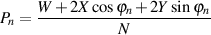 | (10.33) |
Where
Pn is the amplitude of the nth loudspeaker, φn is the angle of the nth loudspeaker in the listening room, and N is the number of loudspeakers.
The decoding algorithm used here is one suggested by Vanderkooy and Lipshitz
which differs from Gerzons original equations in that it uses a gain of 2 on the X and Y
channels rather than the standard  . This is due to the fact that this method omits the 1
gain from
. This is due to the fact that this method omits the 1
gain from  the W channel in the encoding process for simpler analysis [Bamford and
Vanderkooy, 1995].
the W channel in the encoding process for simpler analysis [Bamford and
Vanderkooy, 1995].
 | (10.34) |
Where B is the minimum number of loudspeakers required to accurately produce the panphonic ambisonics signal and m is the order of the system. (So far, we have only discussed first-order Ambisonics in this book.)
Practically speaking, it is difficult to put four microphones (the omnidirectional and the three bidirectionals) in a single location in the recording space. If you’re doing a panphonic recording, you can make a vertical array with the omni in between the two bidirectionals and come pretty close. There is also the small problem of the fact that the frequency responses of the bidirectionals and the omni won’t match perfectly. This will make the contributions of the pressure and the velocity components frequency-dependent when you mix them to send to the loudspeakers.
So, what we need is a smarter microphone arrangement, and at the same time (if we’re smart enough), we need to match the frequency responses of the pressure and velocity components. It turns out that both of these goals are achievable (within reason).
We start by building a tetrahedron. If you’re not sure what that looks like, don’t panic. Imagine a pyramid made of 4 equilateral triangles (normal pyramids have a square base – a tetrahedron has a triangular base). Then we make each face of the tetrahedron the diaphragm of a cardioid microphone. Remember that a cardioid microphone is one-half pressure and one-half velocity, therefore we have matched our components (in theory, at least...). We have cardioids pointing in the directions Left Front (LF) pointing upwards, Right Front (RF) pointing downwards, Left Back (LB) pointing downwards, and Right Back (RB) pointing upwards.
This arrangement of four cardioid microphones in a single housing is what is typically called a soundfield microphone. Various versions of this arrangement have been made over the years by different companies.
The signal consisting of the outputs of the four cardioids in the soundfield microphone make up what is commonly called an A-Format Ambisonics signal. These are typically converted into the B-Format using a standard set of equations given below [Rumsey, 2001].
There are some problems with this implementation. Firstly, we are oversimplifying a little too much when we think that the four cardioid capsules can be combined to give us a perfect B-Format signal. This is because the four capsules are just too far apart to be effective at synthesizing a virtual omni or bidirectional at high frequencies. We can’t make the four cardioids coincident (they can’t be in exactly the same place) so the theory falls apart a little bit here – but only for high frequencies. Secondly, nobody has ever built a perfect cardioid that is really a cardioid at all frequencies. Consequently, our dream of matching the pressure and velocity components falls apart a bit as well.
Finally, there’s a strange little problem that typically gets glossed over a bit in most discussions of soundfield microphones. You’ll remember from earlier in this book that the output of a velocity transducer has a naturally rising response of 6 dB per octave. In other words, it has no low-end. In order to make bidirectional (as well as all other directional) microphones sound better, the manufacturers boost the low end using various methods, either acoustical or electrical. Therefore, an off-the-shelf bidirectional (or cardioid) microphone really doesn’t behave “correctly” to be used in a theoretically “correct” Ambisonics system – it simply has too much low-end (and a messed-up low-frequency phase response to go with it...). The strange thing is that, if you build a system that uses “correct” velocity components with the rising 6 dB per octave response and listen to the output, it will sound too bright and thin. In order to make the Ambisonics output sound warm and fuzzy (and therefore good) you have to boost the low-frequency components in your velocity channels. Technically, this is incorrect, however, it sounds better, so people do it.
Ambisonics is a systems that works on “orders” – the higher the order of the system, the more accurate the reproduction of the sound field.
Second-order periphonic
 | (10.44) |
Let’s take a simple 1st-order panphonic Ambisonics system. We can use the equations given above to think of the system in a more holistic way. If we combine the sensitivity equations for the B-format signal with the mix equation for a loudspeaker in the playback system, we can make a plot of the gain applied to a signal as a function of the relationship between the angle to the sound source and the angle to the loudspeaker. That function looks like the graph in Figure 10.151.
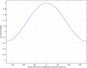
So far, we have been considering the sound from a source recorded by a microphone at a single point in space, played back over loudspeakers and analyzed at a single point in space (the sweet spot). In doing this, we have found out that the soundfield at the sweet spot exactly matches the soundfield at the sweet spot within the constraints of the order of the Ambisonics system.
Let’s now change the analysis to consider what you actually hear. Instead of a single-point microphone, you have two ears, one on either side of your head. Let’s look at two situations, a sound source directly in front of you and a sound source directly to the side. To simplify things, we’ll put ourselves in an anechoic world.
As we have already seen, a Head Related Transfer Function (or HRTF) is a description of what your head and ears do to a sound signal before hitting your eardrum. These HRTF’s can be used in a number of ways, but for our purposes, we’ll stick to impulse responses, showing what’s happening in the time domain. The analysis you’re about to read uses the HRTF database measured at MIT using a KEMAR dummy head. This is a public database available for download via the Internet[Gardner and Martin, 1995].
We’ll begin by looking at the HRTF’s of two sound sources, one directly in front of the listener and one directly to the right. The impulse responses for the resulting HRTF’s for these two locations are shown in Figures 10.152 and 10.153 respectively.
There are two things to notice about the two impulse responses shown in Figure 10.152 for a frontal sound source. Firstly, the times of arrival of the impulses at the two ears are identical. Secondly, the impulse responses themselves are identical throughout the entire length of the measurement.
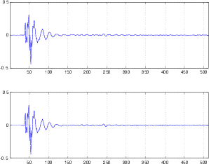
Let’s consider the same two aspects for Figure 10.153 which shows the HRTF’s for a sound source on the side of a listener. Notice in this case that the times of arrival of the impulses at the two ears different. Since the sound source is on the right side of the listener, the impulse arrives at the right ear before the left. This makes sense since the right ear is closer to sound sources on the right side of your head. Now take a look at the impulse response over time. The first big spike in the right ear goes positive. Similarly, the first big spike in the left ear also goes positive. This should not come as a surprise, since your eardrums are not bidirectional transducers. These interaural time differences (ITD’s) are very significant components that our brains use in determining where a sound source is.
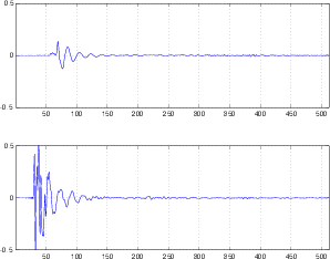
Let’s now consider a source directly in front of a soundfield microphone, recorded in 1st-order Ambisonics and played over an 8-channel loudspeaker configuration shown in Figure 10.154.
If we assume that the sound source emits a perfect impulse and is recorded by a perfect soundfield microphone and subsequently reproduced by 8 perfect loudspeakers, we can use the same HRTF measurements to determine the resulting signal that arrives at the ears of the dummy head. Figure 10.155 shows the HRTF’s for a sound source recorded and reproduced through such a system. Again, let’s look at the same two characteristics of the impulse responses. The times of arrival of the impulse at the two ears are identical, as we would expect for a frontal sound source. Also, the two impulse responses are identical, also expected for a frontal sound source. So far, Ambisonics seems to be working... however, you may notice that the impulse responses in Figure 10.155 aren’t identical to those in Figure 10.152. Frankly, however, this doesn’t worry me too much. We’ll move on...
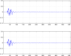
Figure 10.156 shows the HRTF’s for a sound source 90∘ off to the side of a soundfield microphone and reproduced through the same 8-channel Ambisonics system. Again, we’ll look at the same two characteristics of the impulse responses. Firstly, notice that the times of arrival of the pressure waves at the two ears is identical. This contrasts with the impulse responses in Figure 10.153. The interaural time differences that occur with real sources are eliminated in the Ambisonics system. This is caused by the fact that the soundfield microphone cannot detect time of arrival differences because it is in one location.
Secondly, notice the differences in the impulse responses at the two ears. The initial spike in the right ear is positive whereas the first spike in the left ear is negative. This is caused by the fact that loudspeakers that are opposite each other in the listening space in a 1st-order Ambisonics system are opposite in polarity. This can be seen in the sensitivity function shown in Figure 10.151. The result of this opposite polarity is that sound sources on the sides sound similar to a stereo signal normally described as being “out of phase” where the two channels are opposite in polarity [Martin et al., 1999].
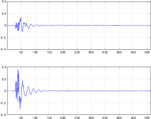
In the interest of fairness, a couple of things should be pointed out here. The first is that these problems are most evident in 1st-order Ambisonics systems, The higher the order, the less problematic they are. However, for the time being, it is impossible to do a recording in a real space in any Ambisonics system higher than 1st-order. Work has been done to develop coefficients that avoid polarity differences in the system [Malham, 1999] and people are developing fancy ways of synthesizing higher-order directional microphones using multiple transducers, however, these systems have associated problems that will not be discussed here.
Microphone techniques for surround sound are still in their infancy. I suppose that, if you really wanted to argue about it, you could say that stereo microphone techniques are as well, but at least we’ve all had a little more experience with two channels than five.
As a result, Most of what is contained in this chapter is basically just a list of some suggested configurations from various people along with a lot of my own opinions. Someday, in the future, I plan on adding an additional chapter to this book that is the surround equivalent to Section 10.4 (Although you should note that there is some information in there as well on surround.).
The goal in surround recording is basically the same as it is for two-channel. You have to get a pretty (or at least desired) timbral and spatial representation of your ensemble to the end listener. The good thing about surround is that your possibilities for spatial effects are much greater than they are with stereo. We could make a case for realism – a “you-are-there” representation of the ensemble, but I’m not one of the people that belongs to this camp, so I won’t go there.
If you’ve one of the many people that has only heard a couple of surround sound recordings, you are probably questioning whether it’s really worth all the trouble to record in surround. Many, if not most of the surround recordings available for consumption are bad examples of the capabilities of the system. Don’t despair – the problem lies in the recordings, not surround itself. You have to remember that everyone’s just in the learning process of what to do with surround. Also, keep in mind that surround is still new, so everyone is doing fairly gimmicky recordings. Things that show off individual characteristics of the system instead of trying to do a good recording. (For example, it’s easy to tell when a studio buys a new reverb unit because their next two releases have tons of reverb in them.) There are many exceptions to this broad criticism of surround recordings, but I won’t mention any names, just in case I get myself in trouble.
There are many reasons to upgrade to surround recordings. the biggest reason is freedom – surround allows you much more room to use spatial characteristics of the distribution medium as a creative tool in your recordings.
There is a lot of debate in the professional community regarding whether or not to use the centre channel. Most people think that it’s a necessary component in a surround system in order to have a larger listening area. There is a small, but very vocal group that it absolutely dead set against the centre channel, arguing that a phantom centre sounds better (for various reasons, the most important of which is usually timbre).
Here I would like to categorically state a personal opinion that I belong to both camps. The centre channel can very easily be mis-used and, as a result, ruin an otherwise good recording. On the other hand, I have heard some excellent surround recordings that use the centre channel. My personal feeling is that the centre speaker should be used as a spatial tool. A phantom centre and a real centre are very different beasts – use the one you prefer at the moment in your recording where it is most appropriate.
The title of this is pretty obvious... One of the best reasons to use surround sound is that you can have sound that surrounds. I don’t know if I have to say anything else. It is, of course, extremely difficult to have a completely enveloping soundfield for a listener using 2-channel stereo. It’s not easy to do this in 5-channel surround, but it’s easier than it is with stereo.
Believe it or not, if you do a surround recording, it is more likely that your end listeners have a reasonably correct speaker configuration than if you’re working in 2-channel stereo. Think of all your friends (this is easier to do if you think of them one-by-one, particularly if some of them don’t get along...). Of these people, think of the ones with a stereo system. How many of these people have a “correct” loudspeaker configuration? I will bet that the number is very close to none. Now think of people with a surround sound system. In most cases, they have this system for watching movies – so they’ve got a television which is the centre channel (or there’s a small speaker on top), a speaker on either side and a couple of speakers in the rear. Okay, so the configuration probably doesn’t conform to the ITU-775[ITU, 1994] standard, but it’s better than having a stereo system where the left speaker is in the living room and the right speaker is in the kitchen.
Go to an orchestra concert and sit in a front row. Try to listen to the oboe when everyone else is playing and you’ll probably find that you’re able to do this pretty easily. If you could wind back time, you would find that you could have listened to the clarinet instead. (If you don’t like orchestral music, go to a bar and eavesdrop on people’s conversations – you can do this too. If you get caught, tell them it’s research.) You’re able to do this because you are able to track both the timbre and the location of a sound source. (Check out a phenomenon called the cocktail party effect for more information on this.)
If you record in mono, you have to be very careful about your mix. You have to balance all the components very precisely to ensure that people can hear what is needed to be heard at that particular moment. This is because people are unable to use spatial cues to determine where instruments are and therefore devote more concentration to them.
If we graduate to 2-channel stereo, life gets a little easier. By panning sources across the stereo sound stage between the two speakers, people are able to concentrate on one instrument and effectively attenuate others within their brains.
The more spatial cues you give to the listener, the better able they are to effectively zero in on whatever component of the recording they like. This doesn’t necessarily mean that their perception can’t be manipulated but it also means that you don’t have to do as much manipulation in your mixes. Mastering engineers such as Bob Ludwig also report that they are finding that less compression and sweetening is required in surround sound media for the same reasons.
Back in the old days, we used level almost exclusively to manipulate people’s attention in a mix. Nowadays, with surround, you can use level, but also spatial cues to draw attention towards or away from components.
Of course, every silver cloud has a dark lining... Recording in surround doesn’t automatically fix all of your problems and make you a great recording engineer. In fact, if you’re a bad engineer in 2-channel stereo, you’ll be 2.5 times worse in 5-channel (2.55 times worse in 5.1) so be careful.
I would also go so far as to create an equation which I, in a pathetic stab at immortality, will dub Martin’s Law which states that the difficulty of doing a recording and mix in surround sound can be calculated from the number of channels in your media, using Equation 10.45.
 | (10.45) |
where Dris is the Difficulty of Recording in Surround, n is the number of channels in your recording and ref is the number of channels in the media to which you’re comparing. For example, you can calculate that it is 118.4 times more difficult to record in 5.1 than in 2-channel stereo.
You may notice that I used this same topic as one of the advantages for recording in surround. I put it here to make you aware that you shouldn’t just go putting things in the centre channel all willy-nilly. Use the centre channel with caution. Always remember that it’s much easier to localize a real source (like a loudspeaker) in a real room than it is to localize a phantom source. This means that if you want to start playing with people’s perception of distance to the sound source, you might want to carefully consider the centre channel.
Another possible problem that the centre channel can create is in timbre. Take a single channel of pink noise and send it to your Left and Right speakers. If all goes well, you’ll get a phantom centre. Now, move around the sweet spot a bit and listen to the timbre of the noise. You should hear some comb filtering, but it really shouldn’t be too disturbing. (Now that you’ve heard that, listen for it on the lead vocals of every CD you own... Sorry to ruin your life...) Repeat this experiment, but this time, send the pink noise to the Centre and Right channels simultaneously. Now you should get a phantom image somewhere around 15∘ off-centre, but if you move around the sweet spot you’ll hear much more serious problems with your comb filtering. This is a bigger problem than in stereo because your head isn’t getting in the way of the signal from the Centre speaker. In the case of Left interfering with Right, you have a reasonably high degree of attenuation in the crosstalk (Left speaker getting to the right ear and vice versa.) In the case of the Centre channel, this attenuation is reduced, so you get a big interference between the Centre and Right channels in your right ear. The left ear isn’t a problem because the Right channel is attenuated. So, the moral of this story is to be careful with sources that are panned between speakers – decide whether you want the comb filtering. It’s okay to have it as long as it’s intentional [Martin, 2002a][Martin, 2002b].
So, going back to my statement in the previous section... The centre channel itself is not a problem, it’s in the way you use it. Centre channels don’t kill recordings, recording engineers kill recordings.
Don’t expect perfect localization for all sources, 360∘ around the listener. A single, focused phantom image on the side is probably impossible to achieve. Phantom images behind the listener appear to get very close, sometimes causing in-head localization. (Remember that the surround channels are basically a giant pair of headphones.) Rear images are highly unstable and dependent on the listeners movements due to the wide separation of the loudspeakers.
Note that if you want to search for the holy grail of stable, precise and accurate side images, you’ll probably have to start worrying about the spatial distribution and timing of your early reflections [Lund, 2000].
If you watch a movie mixed by a bad re-recording engineer (the film world’s equivalent of a mixing engineer in the music world), you’ll notice a couple of obvious things. All of the dialog and foley (all of the little extra sound effects like zipping zippers, stepping foot steps and shutting doors) comes from the Centre speaker, the music comes from the Left and Right speakers, and the Surround speakers are used for the occasional special effect like rain sounds or crowd noises. Essentially, you’re presented with three completely unrelated soundfields. You can barely get away with this independence of signal in a movie because people are busy using their eyes watching beautiful people in car chases. In music-only recordings, however, we don’t have the luxury of this distraction, unfortunately.
Listen to a poorly-recorded or mixed surround recording and you’ll notice a couple of obvious, but common, mistakes. There is no connection between the front and surround speakers – instruments in the front, reverb in the surround is a common presentation that comes from the film world. Don’t get me wrong here, I’m not saying that you shouldn’t have a presentation where the instruments are in the front only – if that’s what you want, that’s up to you. What I’m saying is, if you’re going for that spatial representation, it’s a bad idea to use your surrounds as the only reverb in the mix. They’ll sound completely disconnected with your instruments. You can correct this by making some of the signals in the front and the rear the same – either send instruments to the rear or send reverb to the front. What you do is up to you, but please be careful to not have a large wall between your front and your rear. This is the surround equivalent of some of the early days of stereo where the lead vocals were on the left and the guitar on the right. (Not that I don’t like the Beatles, but their early stereo recordings weren’t exactly sophisticated, spatially speaking...)
This may initially seem like a rather personal question, but it really isn’t, I assure you.
Take some pink noise and send it to all 5 channels in your surround system. Start at the sweet spot and move around just a little – you’ll notice some pretty horrendous comb filtering. If you move more, you’ll notice that the noise collapses pretty quickly to the nearest speaker. This is normal – and the more absorptive your room, the worse it will be. Now, send a different pink noise generator to each of your five channels. (If you don’t have five pink noise generators lying around, you can always just use big delays on the order of a half second or so. So you have the pink noise going to Left, then Centre a half-second later, and Right a half-second after that and so on around the room...) Now you’ll notice that if you move around the sweet spot, you don’t get any comb filtering. This is because the signals are too different to interfere with each other. Also, big movements will result in less collapse to a speaker. This is because your brain is getting multiple different signals so it’s not trying to put them all together into one single signal.
The moral of this story is that, if you want a bigger sweet spot, you’re going to have to make the signals in the speakers different. (In technical terms, you’re looking for decorrelation between your channels. This is particularly true of reverberation. The easiest way to achieve this with microphone technique is to space your microphones. The farther apart they are, the less alike their signals as was discussed earlier.
This is a common error that many people make. If you take a look at the official standard for a 5-channel loudspeaker configuration shown earlier, you’ll see that the surround loudspeakers are to be placed in the 100∘ - 120∘ zone. Typically, people like to use the middle of this zone - 110∘, but lots of pop people like pushing the surrounds a little to the rear, keeping them at 120∘.
Be careful not to think of the surround loudspeakers as rear loudspeakers. They’re really out to the sides, and a little to the rear, they’re not directly behind you. This becomes really obvious if you try to create a phantom centre rear image using only the surround channels. You’ll find in this case that the apparent distance to the sound source is quite close to the back of your head, but this is not surprising if you draw a straight line between your two surround loudspeakers... In theory, of course, the apparent distance to the source should remain constant as it pans from LS to RS, but this is not the case, probably because the speakers are so far apart,
This configuration, developed by Akira Fukada at NHK Japan was one of the first published recommendations for a microphone technique for ITU-775 surround [Fukada et al., 1997]. As can be seen in Figure 10.157, it consists of five widely spaced cardioids, each sending a signal to a single channel. In addition, two omnidirectional microphones are placed on the sides with each signal routed to two channels.
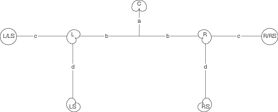
This is a very useful technique, particularly in larger halls with big ensembles. The large separation of the front three cardioids prevents any detrimental comb filtering effects in the listening room on the direct sound of the ensemble (this problem is discussed above). One interesting thing to try with this configuration is to just listen to the five cardioid outputs with a large distance to the rear microphones. You will notice that, due to the large separation between the front and rear signals in the recording space, the perceived sound field in the listening room has two separate areas – that is to say that the frontal sound stage appears to be separate from the surround with nothing connecting them. This is caused by the low correlation between the front and rear signals. Fukada cures this problem by sending the outputs of the omnis to front and surround. The result is a very spacious soundfield, but with reasonably reliable imaging characteristics. You may notice some comb filtering effects caused by having identical signals in the L/LS and R/RS pairs, but you will have to listen carefully for them...
Notice that the distance between the front array and rear pair of microphones can be as little as 0 m, therefore, there may be situations where all microphones but the centre are placed on a single boom.
NOT YET WRITTEN
NOT YET WRITTEN
NOT YET WRITTEN
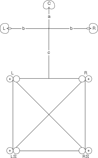
John Klepko developed an interesting surround microphone technique as part of his doctoral work at McGill University [Klepko, 1997]. He suggests that the surround loudspeakers, due to their inherent low interaural crosstalk, can be considered as a very large pair of headphones and could therefore be used to reproduce a binaural signal. Consequently, he suggests that the surround microphones be replaced by a dummy head placed approximately 1.25 metres behind the front microphone array of three hypercardioids spaced at 17.5 cm apart each, and with the L and R microphones aimed ±30∘.
This is an interesting technique in its ability to create a very coherent soundfield that envelops the listener, both left to right and front to back. Part of the reason for this is that the binaural signal played through the surround channels is able to deliver a frontal image in many listeners, even in the absence of signals in the front loudspeakers.
Of course, there are some problems with this configuration, in particular caused by the reliance on the binaural signal. In order to provide the desired spatial cues, the listener must be located exactly in the sweet spot between the surround loudspeakers. Movements away from this position will cause the binaural cues to collapse. In addition, there are timbral issues to consider – dummy heads typically have very strong timbral effects on your signal which are frequently not desirable.
This section was originally published by www.dpamicrophones.com under the title “Description of a 5-channel microphone technique” and presented at the 19th International Conference of the Audio Engineering Society in Banff, Alberta, in June, 2003. Thanks to Jason Corey, the co-author of this section, for permission to copy it here in this section.
There are a number of issues to consider when recording for surround sound. Not only do we want to optimize imaging and image location, but also the smooth and even distribution of the reverberation around the listener and a cohesion of the front and back components of the sound field. The main idea behind a 5-channel microphone technique is to capture the entire acoustic sound field, rather than to simply present the instruments in the front and the reverb in the surrounds.
In order to consider the response of a microphone array, we must first consider the response of the playback system. It is important to remember that the response of the front and rear loudspeakers are very different at the listening position. For example, there is far more interference at the ears of the listener between the signals from the Centre and Left or Left and Left Surround loudspeakers than there is between the signals from the Left and Right, or Left Surround and Right Surround drivers. The principal result of this interference is a comb filter effect caused by the lack of attenuation provided by head shadowing.
In order to reduce or eliminate this comb filtering, the microphone array must ensure that the signals produced by some pairs of loudspeakers are different enough to not create a recognizable interference pattern. This is most easily achieved by separating the microphones, particularly the pairs that result in high levels of mutual interference. At the same time, however, you must ensure that the signals are similar enough that a coherent sound field is presented. If the microphone separation is too great, the result is five completely unrelated recordings of the same event, which eliminates the sound image continuity or fusion between channels. With optimal microphone spacing, the signals from the five loudspeakers work together to form a single coherent sound field and we no longer hear them as five individual signals.
This tree was developed using an adequate separation between specific pairs of microphones to prevent interchannel interference. At the same time, it relies on the response of the loudspeakers at the listening position to permit closer spacing, and therefore a smoother distribution of the sound field for the rear pair of microphones. The configuration consists of three front-facing subcardioids and two ceiling facing cardioid microphones as is shown in Figure 10.162. The approximate dimensions of the array is 60 cm between the Centre subcardioid and the left and Right subcardioids, 60 cm between the front microphones and the surround pair, and 30 cm between a pair of cardioid microphones aimed upwards. If desired, the Centre microphone can be moved slightly forward of the Left and Right mics to an approximate maximum of 15 cm.
A subcardioid microphone is theoretically equivalent to coincident cardioid and omnidirectional microphones whose signals are mixed at equal levels. By using subcardioid microphones we are getting a wider pick-up than is typical with cardioid mics, with a higher directivity than omnidirectional mics. In this way, the microphones can be placed further away from the ensemble than omnidirectional microphones for an equivalent direct to- reverberant ratio. The important point is that we still want to have a certain amount of diffuse, reverberant sound in the front channels that will blend with the direct sound and with the reverberant signals produced by the surround channels. The direct-to-reverberant ratio can be adjusted by changing the distance between the microphone array and the sound source.
The width of the front array is determined by the size of the ensemble being recorded or by the desired level of inter-channel coherence. For a larger ensemble, a wider array (up to 180 cm) is likely necessary. Where a narrow spacing (120 cm) is appropriate for a small ensemble. A wide spacing will reduce the amount of coherence between the front three channels, thereby reducing the image fusion between the loudspeakers. The amount of coherence between the front and surround images can be partly determined by the spacing between the front and rear microphones.
For the surround channels, aiming the surround cardioid microphones to the ceiling has two advantages. Firstly, the direct sound from the ensemble is attenuated because it is arriving near the null of the polar pattern. This is also true of audience noise in the case of a live recording. That being said, any direct sound that is picked up by the surround microphones helps to create some level of coherence between the front and surround channels. The front-back coherence provides an even spread of the sound image along the sides of the loudspeaker array. The level of front-back coherence can be adjusted by changing the angle of the microphones and therefore controlling the amount of direct sound in the surround channels. Secondly, the often ignored vertical dimension of an acoustic space provides diffuse signals that are ideal for the surround channels. For instance, when listening to live music in a concert hall, we hear sound arriving from all directions, not only the horizontal plane.
The microphone array allows for a large listening area in the reproduction system. Even when a listener is seated behind the sweet-spot, the front image of the direct sound will remain in the front and will not be pulled to the rear, despite the listener being closer to the rear loudspeakers.
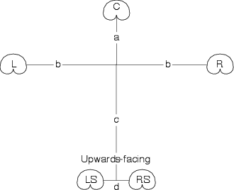
NOT YET WRITTEN
NOT YET WRITTEN - SIMPLIFIED VERSION OF MY BARCELONA AES PAPER
When you tape a show on television, you don’t need to worry about how the sound and the video both wind up on your tape – or how they stay synchronized once they’re both on there – but if you’re working in the television or film industry, this is a very big issue. Usually, in film recording, the audio gets recorded on a completely different machine than the film. In video editing, you need a bunch of video playback and recording units all “synchronized” so that some central machine knows where on the tapes all the machines are – down to the individual frame. How is this done? Well, the location of the tape – the “time” the tape is at – is recorded on the tape itself, so that no matter which machine you play it on, you can tell where you are in the show – to the nearest frame. This is done with what’s called time code of which there are various species to talk about...
Before discussing time code formats, we have to talk about the different frame rates of the various media which use time code. In spite of the original name “moving pictures,” all video and film that we see doesn’t really use pictures that move. We are shown a number of still pictures in quick succession that fool our eyes into thinking that we’re seeing movement. The rate at which these pictures (or “frames”) are shown is called the frame rate. This rate varies depending on what you’re watching and where you live.
The film industry uses a standard frame rate of 24 fps (Frames per Second). This is just about the slowest frame rate you can get away with and still have what appears to be smooth motion. (though some internet video–streaming people might argue that point in their advertising brochures...) The only exception to this rule is the IMAX format which runs at twice this rate – 48 fps.
a.k.a. NTSC (National Television System Committee)
(although some people think it stands for “Never The Same Colour”...)
In North America (or at least most of it...) the AC power that runs our curling irons and golf ball washers (and televisions...) has a fundamental frequency of 60 Hz. As a result, the people that invented black and white television, thinking that it would be smart to have a frame rate that was compatible with this frequency, set the rate to 30 fps.
I should mention a little bit about the way televisions work. They’re slightly different from films in that a film shows you 24 actual pictures on the screen each second. A television has a single gun that creates a line of varying intensity on the screen. This gun traces a bunch of lines, one on top of each other on the screen, that, when seen together, look like a single picture. There are 525 lines in each frame – but each frame is divided into two “fields” – the TV shows you the odd–numbered lines, and then goes back to do the even–numbered ones. This system (of alternating between the odd and even number lines using two fields) is called interlacing. The important thing to remember is that since we have 30 fps and 2 fields per frame, this means that there are 60 fields per second.
It would be nice if B and W and colour could run at the same rate – this would make life simple... unfortunately, however, this can’t be done because colour TV requires that a little more information be sent to your unit than B and W does. They’re close – but not exactly the same. Colour NTSC runs at a frame rate of 29.97 fps. This will cause us some grief later.
a.k.a. PAL (Phase Alternating Line)
and SECAM (Sequential Couleur Avec Memoire or Sequential Colour with Memory)
The Europeans have got this figured out far more intelligently than the rest of us. Both PAL and SECAM, whether you’re watching colour OR B and W, run at 25 fps. (There is one exception to this rule called PAL M – but we’ll leave that out...) The difference between PAL and SECAM lies in the methods by which the colour information is broadcast – but we’ll ignore that too. Both systems are interlaces – so you’re seeing 50 fields per second.
It’s interesting that this rate is so close to the film rate of 24 fps. In fact, it’s close enough that some people, when they’re showing movies on television in PAL or SECAM just play them at 25 fps to simplify things. The audio has to be pitch shifted a bit, but the difference is close enough that most people don’t notice the artifacts.
Time code assumes a couple of things. Firstly, it assumes that there are 24 hours in a day, and that your film or television program won’t last longer than a day. So, you can count up to 24 hours (almost...) before you start counting at 0 again. The time is divided in a similar way to the system we use to tell time, with the exception of the sub–division of the seconds. This is divided in frames instead of fractions, since that’s the way the film or video unit works.
So, a typical time code address will look like this:
01:23:35:19
or
HH:MM:SS:FF
Which means 01 hours, 23 minutes, 35 seconds and 19 frames. The number of frames in each second depends on the time code format, which in turn, depends on the medium for which it’s being used, which is discussed in the next section.
Given the number of different “standard” frame rates, there must be a number of different time code formats correspondingly. Each one is designed to match its corresponding rate, however, there are two that stand out as being the most widely used. These formats have been standardized by two organizations, SMPTE (the Society of Motion Picture and Television Engineers – pronounced SIM–tee) and the EBU (the European Broadcasting Union – pronounced ee–be–you)
As you’ll probably guess, this time code is used in the film industry. The system counts 24 frames in each second, as follows:
00:00:00:00
00:00:00:01
00:00:00:02
.
.
.
00:00:00:22
00:00:00:23
00:00:01:00
00:00:01:01
and so on. Notice that the first frame is labelled “00” therefore we count up to 23 frames and then skip to second 01, frame 00. As was previously mentioned, there are a maximum of 24 hours in a day, therefore we roll back around to 0 as follows:
23:59:59:21
23:59:59:22
23:59:59:23
00:00:00:00
00:00:00:01
and so on.
Each of these addresses corresponds to a frame in the film, so while the film is rolling, out time code reader will display a new address every 24th of a second.
In theory, if our film started exactly at midnight, and it ran for 24 hours, then the time code would display the time of day, all day.
This time code is used with PAL and SECAM television formats. The system counts 25 frames in each second, as follows:
00:00:00:00
00:00:00:01
00:00:00:02
.
.
.
00:00:00:23
00:00:00:24
00:00:01:00
00:00:01:01
and so on. Again, the first frame is labelled “00” but we count to 24 frames before skipping to second 01, frame 00. The roll around to 0 after 24 hours happens the same as the 24 fps counterpart, with the obvious exception that we get to 23:59:59:24 before rolling back to 00:00:00:00.
Again, each of these addresses corresponds to a frame in the video, so while the program is playing, out time code reader will display a new address every 25th of a second.
And again, the time code exactly corresponds to the time of day.
This time code is designed to be used in black and white NTSC television formats, however it’s rarely used these days except in the occasional commercial. The system counts 30 frames in each second corresponding with the frame rate of the format, as follows:
00:00:00:00
00:00:00:01
00:00:00:02
.
.
.
00:00:00:28
00:00:00:29
00:00:01:00
00:00:01:01
and so on.
The question you’re probably asking is ‘why is it called “non–drop?” ‘ but that question is probably best answered by explaining one more format called ‘30 fps “drop–frame” ’
This time code is the one that’s used most frequently in North America – and the one that takes the most dancing around to understand. Remember that NTSC started as a 30 fps format until they invented colour – then things slowed down to a frame rate of 29.97 fps when they upgraded. The problem is, how do you count up to 29.97 every second? Well, obviously, you don’t. So, what they came up with was a system where they’d keep counting with the old 30 fps system, pretending that there were 30 frames every second. This means that, at the end of the day, your clock is wrong – you’re counting too slowly (0.03 fps too slowly, to be precise...), so there’s some time left over to make up for at the end of the day – in fact, when the clock on the wall strikes midnight, 24 hours after you started counting, you’re going to have 2592 frames left to count.
The committee that was deciding on this format elected to leave out these frames in something approaching a systematic fashion. Rather than leave out the 2592 frames at the end of the day, they decided to distribute the omissions evenly throughout the day (that way, television programs of less than 24 hours would come close to making sense...) So, this means that we have to omit 108 frames every hour. The way they decided to do this was to omit 2 frames every minute on the minute. The problem with this idea is that omitting 2 frames a minute means losing too many frames – so they had to add a couple back in. This is accomplished by NOT omitting the two frames if the minute is at 0, 10, 20, 30, 40 or 50.
So, now the system counts like this:
00:00:00:00
00:00:00:01
00:00:00:02
.
.
.
00:00:58:29
00:00:59:00
00:00:59:01
.
.
.
00:00:59:28
00:00:59:29
00:01:00:02 (Notice that we’ve skipped two frame numbers)
00:01:00:03
and so on... but...
00:09:59:00
00:09:59:01
00:09:59:02
.
.
.
00:09:59:28
00:09:59:29
00:10:00:00 (Notice that we did not skip two frame numbers)
00:10:00:01
It’s important to keep in mind that we’re not actually leaving out frames in the video – we’re just skipping numbers... like when you were counting to 100 while playing hide and seek as a kid... 21, 22, 25, 26, 30... You didn’t count any faster, but you started looking for your opponents sooner.
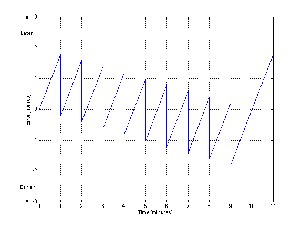
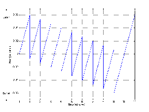
Since we’re dropping out the numbers for the occasional frame, we call this system “drop–frame,” hence the designation “non–drop” when we don’t leave things out.
Look back to the explanation of 30 fps “non–drop” and you’ll see that we said that pretty well the only place it’s used nowadays is for television commercials. This is because the first frame to get dropped in drop–frame happens 1 minute after the time code starts running. Most TV commercials don’t go for longer than 30 seconds, so for that amount of time, drop–frame and non–drop are identical. There is an error accumulated in the time code relative to the time of day, but the error wouldn’t be fixed until the clock read 1 minute anyway... we’ll never get there on a 30–second commercial.
This is a bit of an odd one that’s the result of one small, but very important corner of the video industry – commercials. Commercials for colour NTSC run at a frame rate of 29.97 frames per second, just like everything else on TV – but they typically only last 30 seconds or less. Since the timecode never reaches the 1 minute mark, there’s no need to drop any frames – so you have a frame rate of 29.97 fps, but it’s non–drop.
There are two methods by which the time code signal is recorded onto a piece of videotape, which in turn determine their names. In order to get a handle on why they’re called what they’re called and why they have different advantages and disadvantages, we have to look a bit at how any signal is recorded onto videotape in the first place.
We said that your average NTSC television is receiving 525 lines of information every second – each of these lines is comprised of light and dark areas (or different colours, if your TV is newer than mine...) This means that a LOT of information must get recorded very quickly on the tape – essentially, we require a high bandwidth. This means that we have to run the tape very quickly across the head of the video recorder in order to get everything on the tape. Well, for a long time, we had to do without recorded video because no one could figure out a way of getting the tape–to–head speed high enough without requiring more tape than even a small country could afford... Then one day, someone said “What if we move the head quickly instead of the tape?” BINGO! They put a head on a drum, tilted the drum on an angle relative to the tape and spun the drum while they moved the tape. This now meant that the head was going past the tape quickly, making diagonal streaks across it while the tape just creeped along at a very slow speed indeed.
(Sidebar: the guy in this story was named Alexander M. Poniatoff who was given some cash to figure all this out by another guy named Bing Crosby back in the 40’s... see Bing wanted to tape his shows and then sit at home relaxing with the family while he watched himself on TV... Now, look at Alexander’s initials and tack on an “excellence” and you get AMPEX.)
Back to videotape design... The system with the rotating heads is still used today in your VCR (except that we call it “helical scanning” to sound fancy) and this head on the drum is used to record and play both the video information as well as the “hi–fi” audio (if you own a hi–fi VHS machine). The tape is moving just fast enough to put another head in there which isn’t on the drum – it records the mono audio on your VCR at home, but it could be used for other low–bandwidth signals. It can’t handle high–bandwidth material because the tape is moving so slowly relative to the head that physics just doesn’t allow it.
The important thing to remember from all this is that there are two ways of putting the signal (the time code, in our case) on the tape – longitudinally with the stationary head (because it runs parallel with the tape direction) and vertically with the rotating head (well, it’s actually not completely vertical, but it’s getting close, depending on how much the drum is tilted).
Keep in mind that what we’re discussing here now is how the numbers for the hours, minutes, seconds and frames actually get stored on a piece of tape or transmitted across a wire.
LTC was developed by the SMPTE (which explains the fact that it is occasionally called “SMPTE Time Code” in older books). It is a continuous serial signal with a clock rate of 2400 bits per second and can be recorded on or transmitted through a system with a bandwidth as low as 10 kHz.
The system uses something called bi–phase modulation to encode the numbers into what essentially becomes an audio signal. The numbers denoting the time code address are converted into binary code and then that is converted into the bi–phase mark. “What’s a bi–phase mark?” I hear you cry...
There are a number of ways we can transmit 1’s and 0’s on a wire using voltages. The simplest method would be to assign a voltage to each and send the appropriate voltage at the appropriate time (if I send a 0 V signal – that means 0, but if it’s 1 V, that means 1...) This is a nice system until someone uses a transmission cable that inverts the polarity of the system, then the voltages become 0 V and –1 V – which could be confused for a high and low, then the whole system is screwed up. In order to make the transmission (and recording) system a little more idiot–proof, we use a different system. We’ll keep a high and low voltage, but alternate between them at a pre–determined rate (think square wave). Now the rule is, every transition of the square wave is a new “bit” or number – either a 1 or a 0. Each bit is divided into two “cells” – if there is a voltage transition between cells, then the value of the bit is a 1, if there is no transition between cells, then the bit is a 0 (see the following diagram).
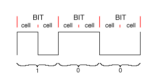
This allows us to invert the polarity and make the voltage of the signal independent of the value of the bit, essentially, making the signal more robust. There is no DC content in the signal (so we don’t have to worry about the signal going through DC–blocking capacitors) and it’s self–clocking (that is to say, if we build a smart receiving device, it can figure out how fast the signal is coming at it). In addition, if we make the receiver a little tolerant, we can change the rate of the signal (the tape speed, when shuttling, for example) and still derive a time code address from it.
Each time code address required one word to define all of its information. This word is comprised of 80 bits (which, at 30 fps means 2400 bits per second). All 80 bits are not required for telling the machines what frame we’re on – in fact only 26 bits are used for this. The rest of the word is divided up as follows:
| Information | Number of Bits |
| Time Address | 26 |
| User Information | 32 |
| Sync Word | 16 |
| Status Information | 5 |
| Unassigned | 1 |
There are a number of texts which discuss exactly how these are laid out in the signal – we won’t get into that. But we should take a quick glance at what the additional parts of the TC word are used for.
The time address information uses 4 bits to encode each of the decimal numbers in the time code address. That is to say, for example, to encode the designation of “12 frames,” the numbers 1 (0001) and 2 (0010) are used sequentially instead of encoding the number 12 as a binary number. This means, in theory, that we require 32 bits to store or transmit the time code address, four bits each for 8 digits (HH:MM:SS:FF). This is not really the case, however, since we don’t count all the way up to 9 with all of the digits. In fact, we only require 2 bits each for the tens of hours (because it never goes past “2”) and tens of frames, and 3 bits for each of the tens of minutes and tens of seconds. This frees up 6 bits which are used for status information, meaning 26 bits are used for the time address information.
There are 32 bits in the time code word reserved for storing what’s called “user information.” These 32 bits are divided into eight 4–bit words which are generally devoted to recording or transmitting things like reel numbers, or the date on which the recording was made – things which don’t change while the time code rolls past. There are two options that are not used as frequently which are:
– encoding ASCII characters to send secret messages (like song lyrics? credits?... be creative...) This would require 8–bit bytes instead of 4–bit words, but we’ll come back to that in the Status Information
– since we have 32 bits to work with, we could lay down a second time code address... though I don’t know what for offhand.
In order for the receiving device to have any clue as to what’s going on, it has to know when the time code word starts and stops, otherwise, its guess is as good as anybody’s. The way the beginning of the word is marked is by putting in a string of bits that cannot happen anywhere else, irrespective of the data that’s being transmitted. This string of data (0011111111111101 to be precise) tells the receiver two things – firstly, where the subsequent word starts (the string is put at the end of each word) and whether the signal is going forwards or backwards. (Notice that the string is two 0’s. twelve 1’s, a 0 and a 1. The receiver sees the twelve 1’s, and looks to see if that string was preceded by two 0’s or a 1 and a 0... that’s how it figures it out.)
The five status bits are comprised of “flags” which provide the receiving device with some information about the signal coming in. I’ll omit explanations for some of these.
If this bit is a 1, then the time code is drop–frame. If it’s a 0, then it’s non–drop.
This is a bit which will change between 0 and 1 depending on the content of the remainder of the word. It’s just there to ensure that the transition at the beginning of every word goes in the same direction.
We said earlier that the User Information is 32 bits divided into eight 4–bit words. However, if it’s being used for ASCII information, then it has to be divided differently into four 8–bit bytes. These User Flags in the Status Information section tell the receiver which system you’re using in the User Information.
This is a bit that has no determined designation.
There’s a couple of little things to know about LTC what might come in useful some day.
Firstly, a time code reader should be able to read time code at speeds between 1/40th of the normal rate and 40 times the normal rate. This would put the maximum bandwidth up to 96000 bits per second (2400 * 40)
Secondly, remember that LTC is recorded using the stationary head on the video recorder. This means a couple of things:
1) as you slow down, you get more inaccurate. If you’re stopped (or paused) you don’t read a signal – therefore no time code.
2) as you slow down, the signal gets lower in amplitude (because the voltage produced by the read head is proportional to the change in magnetism across its gap). Therefore, the slower the tape, the more difficult to read.
Lastly, if you’re using LTC to lock two machines together, keep in mind that the “slave” machine is not locked to every single frame to the closest 80th of a frame to the “master.” In fact, more likely than not, the slave is running on its own internal clock (or some external “house sync” signal) and checking the incoming time code every once and a while to make sure that things are on schedule. (this explains the “forward/backward” info stored in the Sync Word) This can explain why, when you hit STOP on your master machine, it might take a couple of moments for the slave device to realize that it’s time to hit the brakes...
There are two major problems associated with longitudinal time code. Firstly, it is not frame–accurate (not even close...) when you’re moving at very slow speeds, or stopped, as would be the case when shuttling between individual frames (remember that it’s possible to view a stopped frame because the head keeps rotating and therefore moving relative to the tape). Secondly, the LTC takes up too much physical space on the videotape itself.
The solution to both of these problems was presented by Sony back in 1979 in the form of Vertical Interval Time Code or VITC. This information is stored in what is known as the “vertical blanking interval” in each field (we won’t get into what that means... but it’s useful to know that there is one in each field rather than each frame, increasing our resolution over LTC by a factor of 2. It does, however, mean that an extra flag will be required to indicate which field we’re on.
Since the VITC signal is physically located in the vertical tracks on the tape (because it’s recorded by the rotating head instead of the stationary one) it has a number of characteristics which make it differ from LTC.
- Firstly, it cannot be played backwards. Although the video can be played backwards, each field of each frame (and therefore each word of the VITC code) is being shown forwards (in reverse order).
- Secondly, we can trust that the phase of the signal is reliable, so a different binary encoding system is used called Non–Return to Zero or NRZ. In this system, a value of 80 IRE (an IRE is a unit equal to 1/140th of the peak–peak amplitude of a video signal, usually 1 IRE = 7.14 mV, therefore 140 IRE = 1 V) is equal to a binary “1” and 0 IRE is a 0.
– Thirdly, as was previously mentioned, the VITC signal contains the address of a field rather than a frame.
– Finally, we don’t need to indicate when the word starts (as is done by the sync bits in LTC) since every field has only 1 frame associated with it. Since both the field and the word are read simultaneously (they cannot be read separately) we don’t need to know when the word starts... it’s obvious.
Unlike LTC, there are a total of 90 bits in the VITC word, with the following assignments:
| Information | Number of Bits |
| Time Address | 26 |
| User Information | 32 |
| Sync Groups | 18 |
| Cyclic Redundancy Code | 8 |
| Status Information | 5 |
| Unassigned (Field Mark Flag?) | 1 |
In many respects, these bits are the same as their LTC counterparts, but we’ll go through them again anyway.
This is exactly the same as in LTC.
This is exactly the same as in LTC.
Instead of a single big string of binary bits stuck in one part of the word, the Sync Groups in VITC are fit into the information throughout the word. There is a binary “10” located at the beginning of every 10 bits. This information is used to synchronize the word only. It doesn’t need to indicate either the beginning of the word (since this is obvious due to the fact that there is one word “locked” to each field) nor does it need to indicate direction (we’re always going forwards – even when we’re going backwards...)
This is a method of error detection (not error correction).
There are five status information flags, just as with LTC. All are identical to their LTC counterparts with one exception, the Field Mark. Since we don’t worry about phase in the VITC signal, we can leave out the bi–phase correction.
This flag indicates the field of the address.
There is one disadvantage to VITC that makes use of LTC more versatile. Since VITC is buried in the video information recorded by the helical head, it must be recorded simultaneously with the video. It cannot be recorded afterwards. Since LTC is located on a different section of the tape, it can be striped (recorded) onto the tape later without disturbing the video information.
See the information in Table 10.10.
See the information in Table 10.11.