This posting is a simple one… It’s a setup for the next bunch of postings in this series.
In the last posting, we saw that jitter can be separated into two categories, looking at whether the root of the problem is in the time or the amplitude domain.
A different way to categorise jitter is to start by looking at whether the variation in the timing error is random or deterministic.
If the timing error is random, then there is no way of predicting what the error on the next clock “tick” will be. In this case, the error is caused by some kind of random noise (I know – that’s redundant) somewhere in the system.
However, if it’s deterministic, then the timing error will be correlated with some measurable, interfering signal that is not just random.
An Analogy for Obfuscation
One way to think of this is to imagine the sound coming from a poorly-made piece of audio gear.
You’ll hear the signal
you’ll hear some distortion artefacts that are somehow related to the signal
you’ll hear some “hiss”
and you’ll also hear some “hummmm”.
The signal is what you want to hear.
The other three are things-you-don’t-want-to-hear: stuff that would traditionally be included as TDH+N or “total harmonic distortion plus noise”.
The distortion artefacts are things that are unwanted, but somehow related to the signal – so they are not periodic, but they’re deterministic.
The “hiss” is independent noise – a random signal that is added to (but also unrelated to) your signal.
The hum is not random – it’s periodic (meaning that it repeats itself) – and therefore it’s also deterministic.
If you have a digital audio system, it will have jitter (remember – this might not be anything to worry about… sometimes it just doesn’t matter…). The total jitter that it has is the sum result of all of the different types of jitter that contribute to the total. So, in the chart in Figure 1, you can sort of think of each of the black lines as representing “plus signs”. (Only “sort of”, since it depends on exactly what you’re measuring, and for how long…)
My plan is that I’ll address each of these blocks individually in the coming postings in the series.
In the previous posting, I talked a little about what jitter and wander are, and one of the many things that can cause it. The short summary of that posting is:
Jitter and wander are the terms given to a varying error in the clock that determines when an audio sample should (or did) occur.
Note the emphasis on the word “varying”. If the clock is consistently late by a fixed amount of time, then you don’t have jitter or wander. The clock has to be speeding up and slowing down.
One of the ways you can categorise jitter is by separating the problem into two dimensions – phase (or time) and amplitude.
Let’s say that
you have a “square wave” that carries your encoded digital audio signal coming into your device, AND
you are creating a clock “tick” based on the time of the transition between the high and low voltages AND
you are detecting this transition by looking at what time the voltage value crossed the threshold, which is half-way between your high and low voltages
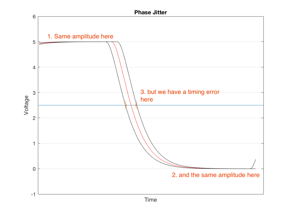
IF there is a variation ONLY in the time that the voltage crossed the threshold – not in the high and low voltage values themselves, then you have what is called phase jitter. This is probably easier to understand if you look at Figure 1, below.
Fig 1. Phase jitter is a “sliding” of the signal in time. The red curve shows when the signal should have crossed the threshold. The black lines show two different errors – one early and one late.
There are three curves in Figure 1. The red curve is the “good” one – it shows the voltage changing from high to low (in this case, 5 V and 0 V), at exactly the right time.
The black curve to the left of this shows an example of a transition that happens too early for some unknown reason. Although that black line also changes from 5 V to 0 V, it does it too early, giving us a timing error when we look at the moment it crosses the threshold (the line at 2.5 V).
The black curve to the right shows an example of a transition that happens too late for some unknown reason. Although that black line also changes from 5 V to 0 V, it does it too late, giving us a timing error when we look at the moment it crosses the threshold (the line at 2.5 V).
As I said above, jitter and wander are the result of a variation in the time that we cross that threshold. So, we will talk about peak-to-peak jitter measurements – a measurement of the amount of time between the earliest detected transition to the latest one. This allows us to not worry so much about measuring a single transition’s error relative to when it should have happened (which would be difficult to do). It’s much easier to just look at the incoming signal over time, and measure the difference in time between the earliest and the latest – the total “width” of the error in time.
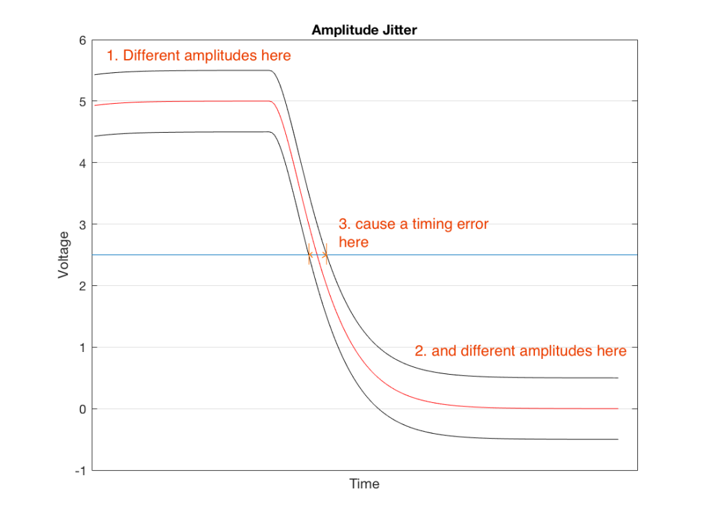
The second classification of jitter is sort of a “side effect” of a different problem. If we take the square wave and we change its amplitude – so we have an error in its voltage level – then a by-product of this is a change in the time the transition crosses the threshold. This is called amplitude jitter and is shown in Figure 2.
Fig 2. Amplitude jitter is an error in the timing caused by an error in the amplitude. The red curve shows when the signal should have crossed the threshold. The black lines show two different errors – one early (because the amplitude was too low) and one late (because the amplitude was too high).
Notice here that the reason the error occurs in time is that we have an error in level. The value of the threshold (the horizontal line at 2.5 V) is based on the assumption that our high and low voltages are 5 V and 0 V. If we have an amplitude error (say, in the case of the upper curve in this plot, 5.5 V and 0.5 V) then the threshold (still at 2.5 V) is too low – so the time the voltage crosses that line will be late.
So, if you have a modulation (a change) in the amplitude (the voltage level) of the signal, then you will also get a modulation in the timing information, resulting in jitter and wander.
Again, this error in time is probably most easily measured as a peak-to-peak jitter value.
Wrapping up
If you’re a system developer or if you’re trying to improve your system, you need to know whether you have phase jitter or amplitude jitter in order to start tracking down the root cause of it so that you can fix it. (If your car doesn’t start and you want to fix it, it’s good to find out whether you are out of fuel or if you have a dead battery… These are two different problems…)
However, if you’re just interested in evaluating the performance of a system, one thing you can do is simply to ask “how much jitter do I have?” (If your car doesn’t start, you’re not going to get to work on time… Whether it’s your battery or your fuel is irrelevant.) You measure this, and then you can make a decision about whether you need to worry about it – whether it will have an effect on your audio quality (which is a question that not determined so much by the amount of jitter that you have, but where it is in your system, and how the “downstream” devices can deal with it).
When many people (including me…) explain how digital audio “works”, they often use the analogy of film. Film doesn’t capture any movement – it’s a series of still photographs that are taken at a given rate (24 frames (or photos) per second, for example). If if the frame rate is fast enough, then you think that things are moving on the screen. However, if you were a fly (whose brain runs faster than yours – which is why you rarely catch one…), you would not see movement, you’d see a slow slide show.
In order for the film to look natural (at least for slowly-moving objects), then you have to play it back at the same frame rate that was used to do the recording in the first place. So, if your movie camera ran at 24 fps (frames per second) then your projector should also run at 24 fps…
Digital audio isn’t exactly the same as film… Yes, when you make a digital recording, you grab “snapshots” (called samples) of the signal level at a regular rate (called the sampling rate). However, there is at least one significant difference with film. In film, if something happened between frames (say, a lightning flash) then there will be no photo of it – and therefore, as far as the movie is concerned, it never happened. In digital audio, the signal is low pass filtered before it’s sampled, so a signal that happens between samples is “smeared” in time and so its effect appears in a number of samples around the event. (That effect will not be part of this discussion…)
Back to the film – the theory is that your projector runs at the same frame rate as your movie camera – if not, people appear to be moving in slow motion or bouncing around too quickly. However, what happens when the frame rate varies a just little? For example, what if, on average, the camera ran at exactly 24 fps, but the projector is somewhat imprecise – so if the amount of time between successive frames varied from 1/25th to 1/23rd of a second randomly… Chances are that you will not notice this unless the variation is extreme.
However, if the camera was the one with the slightly-varying frame rate, then you would not (for example) be able to use the film to accurately measure the speeds of passing cars because the time between photos would not be 1/24th of a second – it would be approximately 1/24th of a second with some error… The larger the error in the time between photos, the bigger the error in our measurement of how far the car travelled in 1/24th of a second.
If you have a turntable, you know that it is supposed to rotate at exactly 33 and 1/3 revolutions per second. However, it doesn’t. It slowly speeds up and slows down a little, resulting in a measurable effect called “wow”. It also varies in speed quickly, resulting in a similar measurable effect called “flutter”. This is the same as our slightly varying frame rate in the film projector or camera – it’s a varying distortion in time, either on the playback or the recording itself.
Digital audio has exactly the same problem. In theory, the sampling rate is constant, meaning that the time between successive samples is always the same. A compact disc is played with a sampling rate of 44100 Samples per Second (or 44.1 kHz), so, in theory, each sample comes 1/44100th of a second after the previous one. However, in practice, this amount of time varies slightly over time. If it changes slowly, then we call the error “wander” and if it changes quickly, we call it “jitter”.
“Wander” is digital audio’s version of “wow” and “jitter” is digital “flutter”.
Transmitting digital audio
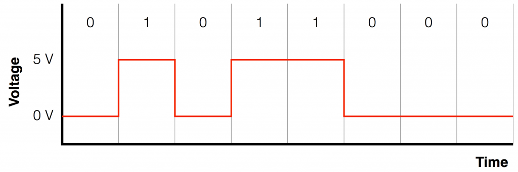
Without getting into any details at all, we can say that “digital audio” means that you have a representation of the audio signal using a stream of “1’s” and “0’s”. Let’s say that you wanted to transmit those 1’s and 0’s from one device to another device using an electrical connection. One way to do this is to use a system called “non-return-to-zero”. You pick two voltages, one high and one low (typically 0 V), and you make the voltage high if the value is a 1 and low if it’s a 0. An example of this is shown in the Figure below.
Fig 1: A binary stream (01011000) transmitted as two voltages using a “non-return-to-zero” protocol. For this example, I used 0 V and 5 V for the “low” and “high” values – the actual voltages are irrelevant.
This protocol is easy to understand and easy to implement, but it has a drawback – the receiving device needs to know when to measure the incoming electrical signal, otherwise it might measure the wrong value. If the incoming signal was just alternating between 0 and 1 all the time (01010101010101010) then the receiver could figure out the timing – the “clock” from the signal itself by looking at the transitions between the low and high voltages. However, if you get a long string of 1’s or 0’s in a row, then the voltage stays high or low, and there are no transitions to give you a hint as to when the values are coming in…
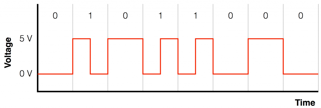
So, we need to make a simple system that not only contains the information, but can be used to deliver the timing information. So, we need to invent a protocol that indicates something different when the signal is a 1 than when it’s a 0 – but also has a voltage transition at every “bit” – every value. One way to do this is to say that, whenever the signal is a 1, we make an extra voltage transition. This strategy is called a “bi-phase mark”, an example of which is shown below in Figure 2.
Fig 2: The same signal, transmitted as a bi-phase mark.
Notice in Figure 2 that there is a voltage transition (either from low to high or from high to low) between each value (0 or 1), so the receiver can use this to known when to measure the voltage (a characteristic that is known as “self-clocking” because the clock information is built into the signal itself). A 0 can either be a low voltage or a high voltage – as long as it doesn’t change. A 1 is represented as a quick “high-low” or a “low-high”.
This is basically the way S-PDIF and AES/EBU work. Their voltage values are slightly different than the ones shown in Figure 2 – and there are many more small details to worry about – but the basic concept of a bi-phase mark is used in both transmission systems.
Detecting the clock
Let’s say that you’re given the task of detecting the clock in the signal shown in Figure 2, above. The simplest way to do this is to draw a line that is half-way between the low and the high voltages and detect when the voltage crosses that line, as shown in Figure 3.
Fig 3: The blue arrows show when the voltage signal crosses the middle line – indicating events that might be used to generate a clock.
The nice thing about this method is that you don’t need to know what the actual voltages are – you just pick a voltage that’s between the high and low values, call that your threshold – and if the signal crosses the threshold (in either direction) you call that an event.
Real-world square waves
So far so good. We have a digital audio signal, we can encode it as an electrical signal, we can transmit that signal over a wire to a device that can derive the clock (and therefore ultimately, the sampling rate) from the signal itself…
One small comment here: although the audio signal that we’re transmitting has been encoded as a digital representation (1’s and 0’s) the electrical signal that we’re using to transmit it is analogue. It’s just a change in voltage over time. In essence, the signal shown in Figure 2 is an analogue square wave with a frequency that is modulating between two values.
Now let’s start getting real. In order to create a square wave, you need to be able to transition from one voltage to another voltage instantaneously (this is very fast). This means that, in order to be truly square, the vertical lines in all of the above figures must be really vertical, and the corners must be 90º. In order for both of these things to be true, the circuitry that is creating the voltage signal must have an infinite bandwidth. In other words, it must have the ability to deliver a signal that extends from 0 Hz (or DC) up to ∞ Hz. If it doesn’t, then the square wave won’t really be square.
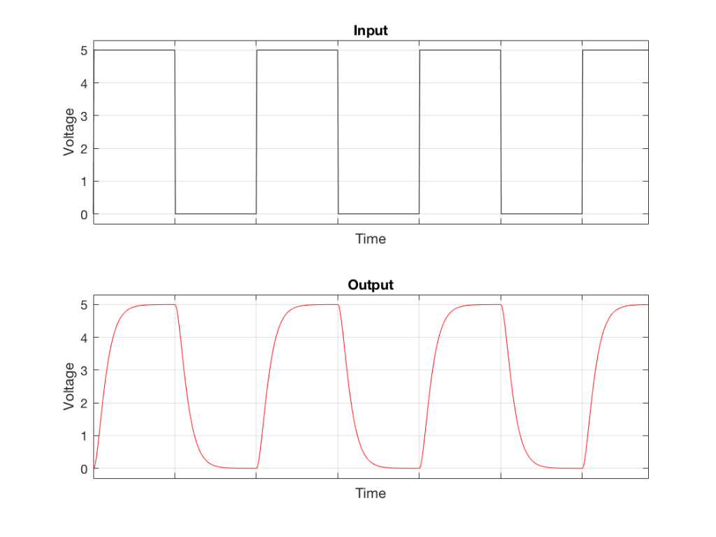
What happens if we try to transmit a square wave through a system that doesn’t extend all the way to ∞ Hz (in other words, “what happens if we filter the high frequencies out of a square wave? What does it look like?”) Figure 4, below shows an example of what we can expect in this case.
Fig 4. The top plot is a square wave. The bottom plot is the result of sending that square wave through a low-pass filter (therefore reducing the high-frequency content). Notice that the 90º angles have been increased a little – and that the vertical transitions are no longer vertical.
Note that Figure 4 is just an example… The exact shape of the output (the red curve) will be dependent on the relationship between the fundamental frequency of the square wave and the cutoff frequency of the low-pass filter – or, more accurately, the frequency response of the system.
What time is it there?
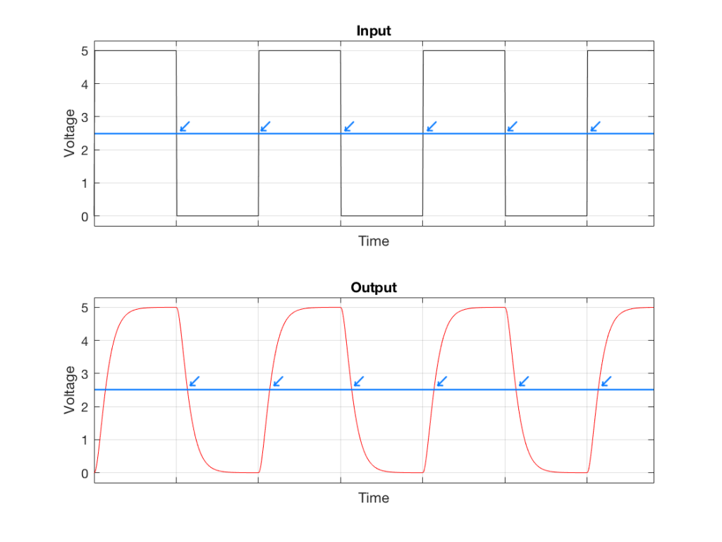
Look carefully at the two curves in Figure 4. The tick marks on the “Time” axes show the time that the voltage should transition from low to high or vice versa. If we were to use our simple method for detecting voltage transitions (shown in Figure 3) then it would be wrong…
Fig 5: The simple method of detecting the transition time results in an error when the square wave isn’t square. Notice that the blue arrows in the lower plot are all late compared to the time when the transition started.
As you can see in Figure 5, the system that detects the transition time is always late when the square wave is low-pass filtered. In this particular case, it’s always late by the same amount, so we aren’t too worried about it – but this won’t always be true…
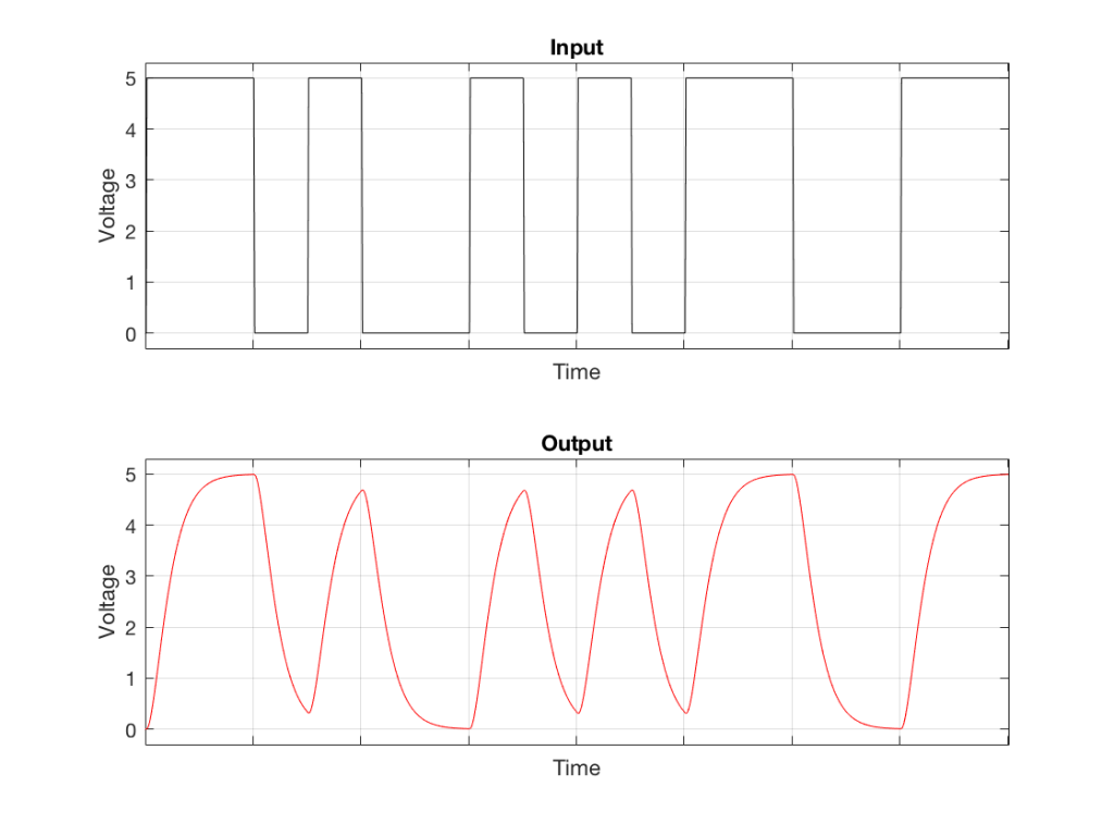
For example, what happens when the signal that we’re low-pass filtering is a bi-phase mark (which means that it’s a square wave with a modulated fundamental frequency) instead of a simple square wave with a fixed frequency?
Fig 6. The top plot shows the same signal plotted in Figure 2 – a bi-phase representation of the binary value 01011000. The bottom plot shows a low-pass filtered version of that signal.
As you can see in Figure 6, the low pass filter has a somewhat strange effect on the modulated square wave. Now, when the binary value is a “1”, and the square wave frequency is high, there isn’t enough time for the voltage to swing all the way to the new value before it has to turn around and go back the other way. Because it never quite gets to where it’s going (vertically) then there is a change in when it crosses our threshold of detection (horizontally), as is shown below.
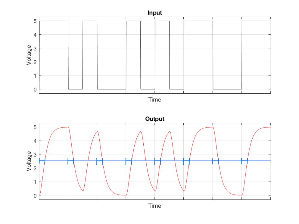
Fig 7: The time that the red plot crosses our threshold is always late – but it’s late by a different amount each time, depending on the signal itself… (In other words, some of those blue H’s are wider than others…)
The conclusion (for now)
IF we were to make a digital audio transmission system AND
IF that system used a biphase mark as its protocol AND
IF transmission was significantly band-limited AND
IF we were only using this simple method to derive the clock from the signal itself
THEN the clock for our receiving device would be incorrect. It would not just be late, but it would vary over time – sometimes a little later than other times… And therefore, we have a system with wander and/or jitter.
It’s important for me to note that the example I’ve given here about how that jitter might come to be in the first place is just one version of reality. There are lots of types of jitter and lots of root causes of it – some of which I’ll explain in this series of postings.
In addition, there are times when you need to worry about it, and times when you don’t – no matter how bad it is. And then, there are the sneaky times when you think that you don’t need to worry about it, but you really do…