Category: audio
Beoplay H6mk2 review

The good ol’ days…
B&O Tech: 100 Years of Danish Loudspeakers
#56 in a series of articles about the technology behind Bang & Olufsen loudspeakers
This book was released some months ago as part of the 100 year anniversary of loudspeaker development in Denmark. There are a number of good articles in there, including a historical article on the importance of loudspeaker directivity at Bang & Olufsen.

Acoustics for vegans
The philosophy of music recording
The Prospects of Recording by Canadian pianist, composer, and broadcaster Glenn Gould makes an interesting read if you the kind of person who debates whether “they” should be “here” or “you” should be “there”.
The Shuffler
For people who are interested in thinking about the concept of stereo, this is a good introduction to one of Blumlein’s original ideas about it called “Stereo Shuffling”.
B&O Tech: A quick primer on distortion
#55 in a series of articles about the technology behind Bang & Olufsen loudspeakers
In a previous posting, I talked about the relationship between its “Bl” or “force factor” curve and the stiffness characteristics of its suspension and the fact that this relationship has an effect on the distortion characteristics of the driver. What was missing in that article was the details in the punchline – the “so what?” That’s what this posting is about – the effect of a particular kind of distortion in a system, and its resulting output.
WARNING: There is an intentional, fundamental error in many of the plots in this article. If you want to know about this, please jump to the “appendix” at the end. If you aren’t interested in the pedantic details, but are only curious about an intuitive understanding of the topic, then don’t worry about this, and read on. As an exciting third option, you could just read the article, and then read the appendix to find out how I’ve been protecting you from the truth…
Examples of Non-linear Distortion
Let’s start by looking at something called a “transfer function” – this is a plot of the difference between what you want and what you get.
For example, if we look at the excursion of a loudspeaker driver: we have some intended excursion (for example, we want to push the woofer out by 5 mm) and we have some actual excursion (hopefully, it’s also 5 mm…)
If we have a system that behaves exactly as we want it to within some limit, and then at that limit it can’t move farther, we have a system that clips the signal. For example, let’s say that we have a loudspeaker driver that can move perfectly (in other words, it goes exactly where we want it to) until it hits 5 mm from the rest position (either inwards or outwards). In this case, its transfer function would look like Figure 1.
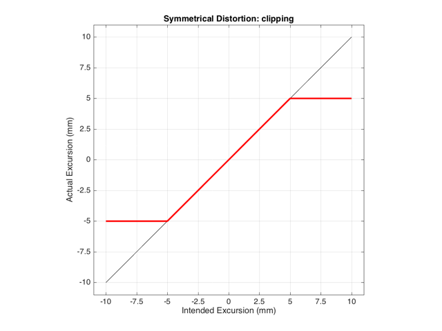
This means that if we try to move the driver with a sinusoidal wave that should peak at 10 mm and -10 mm, the tops and bottoms of the wave will be “chopped off” at ±5 mm. This is shown in Figure 2, below.
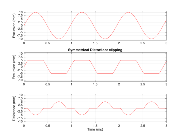
Let’s think carefully about the bottom plot in Figure 2. This is the difference between the actual excursion of the driver and the desired excursion (I calculated it by actually subtracting the top plot from the middle plot) – in other words, it’s the error in the signal. Another way to think of this is that the signal produced by the driver is what you want (the top plot) PLUS the error (the bottom plot). (Looking at the plots, if middle-top = bottom, then top+bottom = middle)
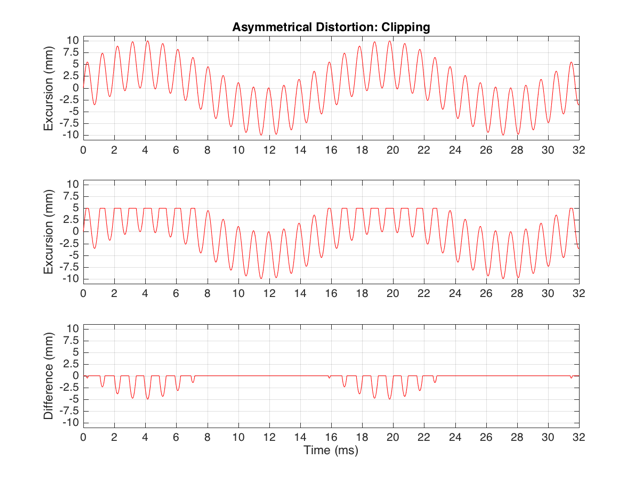
These plots show a rather simple case where the clipping of the signal is symmetrical. That is to say that the error on the positive part of the waveform is identical to that on the negative part of the waveform. As we saw in this posting, however, perfectly symmetrical distortion is not guaranteed… So, what happens if you have asymmetrical distortion? Let’s say, for example, that you have a system that behaves perfectly, except that it cannot move more than 5 mm outwards (moving inwards is not limited). The transfer function for this driver would look like Figure 3.
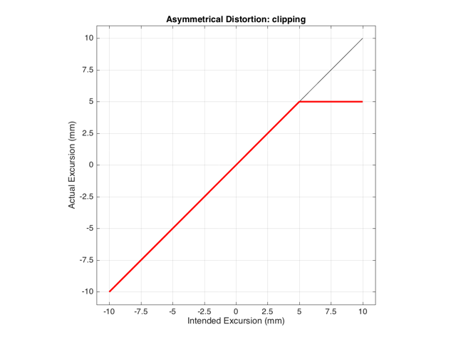
How would a sinusoidal waveform look if it were passed through that driver? This is shown in Figure 4, below.
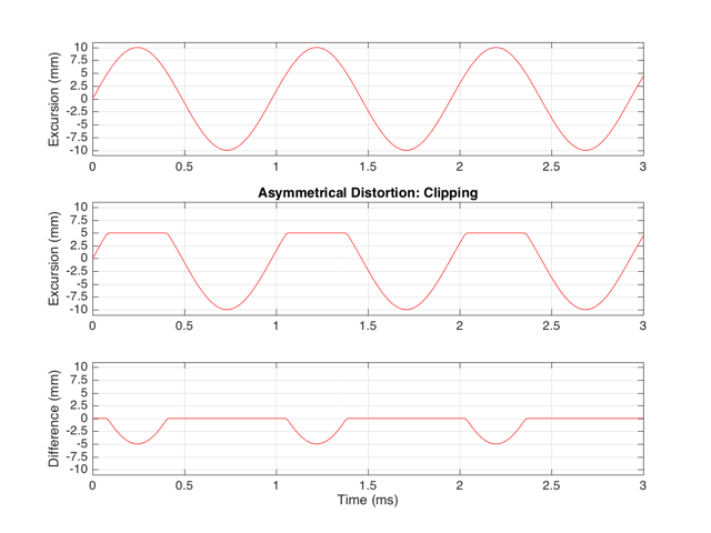
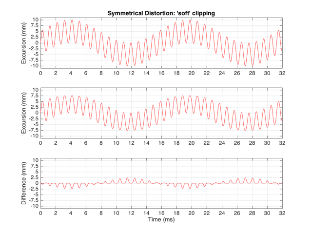
As we also saw before, it is unlikely that the abrupt clipping of a signal is how a real driver will behave. This is because, usually, a driver has an increasing stiffness and a decreasing force to push against it, as the excursion increases. So, instead of the driver behaving perfectly to some limit, and then clipping, it is more likely that the error is gradually increasing with excursion. An example of this is shown below in Figure 5. Note that this plot is just a tanh (a hyperbolic tangent) function for illustrative purposes – it is not a measurement of a real loudspeaker driver’s behaviour.
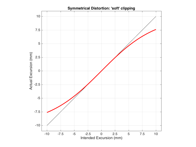
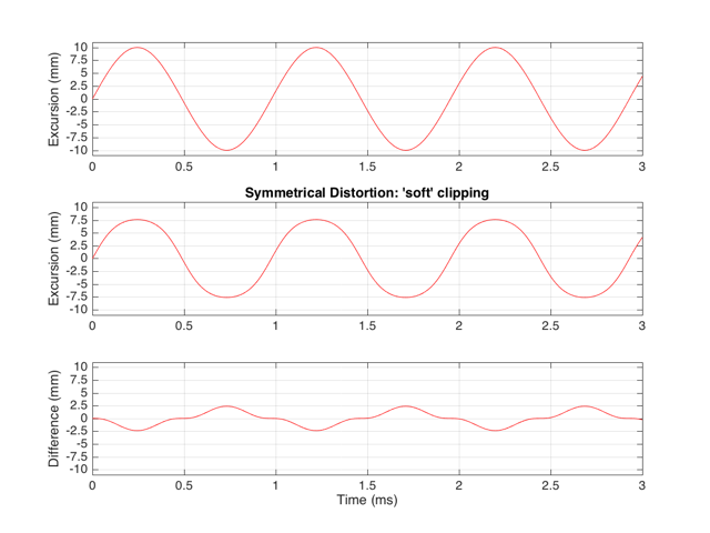
If we were to pass a sinusoidal waveform through this system, the result would be as is shown in Figure 6.
Harmonic Distortion
The reason engineers love sinusoidal waveforms is that they only contain one frequency each. A 1000 Hz sine tone only has energy at 1000 Hz and no where else. This means that if you have a box that does something to audio, and you put a 1000 Hz sine tone into it, and a signal with frequencies other than 1000 Hz comes out, then the box is distorting your sine wave in some way.
This was a very general statement and should be taken with a grain of salt. A gain applied perfectly to a signal is also a distortion (since the output is different from the input), but will not necessarily add new frequency components (and therefore it is linear distortion, not non-linear distortion). A box that adds noise to the signal is, generally speaking, distorting the input – but the output’s extra components are unrelated to the input – which would classify the problem as noise instead of distortion.) To be more accurate, I would have said that “if you have a box that does something to audio, and you put a 1000 Hz sine tone into it, and a signal with frequencies other than 1000 Hz comes out, then the box is applying a non-linear distortion to your sine wave in some way.”
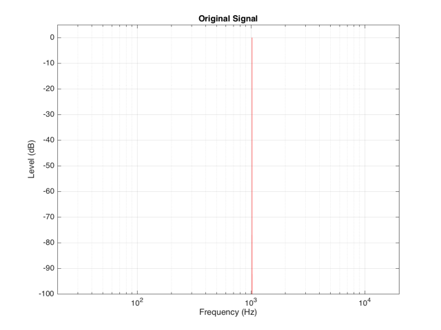
Back to the engineers… If you take a sinusoidal waveform and plot its frequency content, you’ll see something like Figure 7. This shows the frequency content of a signal consisting of a 1024 Hz sine wave.
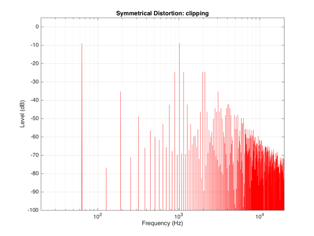
If we clip this signal symmetrically, using the transfer function shown in Figure 1, resulting in the signal shown in the middle plot in Figure 2, and them measure the frequency content of the result, it will look like Figure 8.
There are at least two interesting things to note about the frequency content shown in Figure 8.
The first is that the level of the signal at the fundamental frequency “f” (1024 Hz, in this case) is lower than the input. This might be obvious, since the output cannot “go as loud” as the input of the system – so some level is lost. (Since we’re clipping at -6 dB, the fundamental has dropped by 6 dB.)
The second thing to notice is that the new frequencies that have appeared are at odd multiples of the frequency of the original signal. So, we have content at 3072 Hz (3*1024), 5120 Hz (5*1024), 7168 Hz (7*1024) and so on. This is a characteristic of a symmetrically distorted signal (meaning not only that we have distorted the top and the bottom of the signal in the same way, but also that the signal itself was symmetrical to begin with). In other words, whenever you see a distortion product that only produces odd-order harmonics of the fundamental, you have a system that is distorting a symmetrical signal symmetrically.
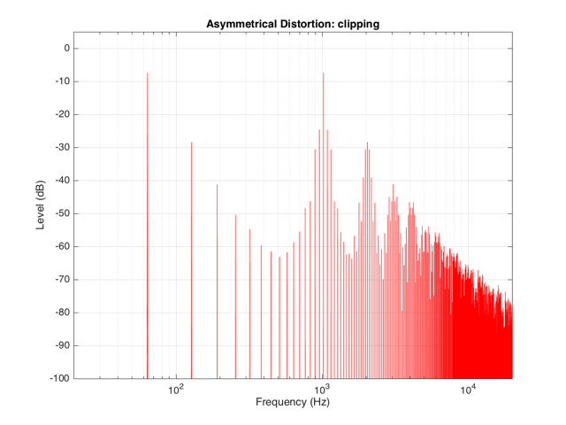
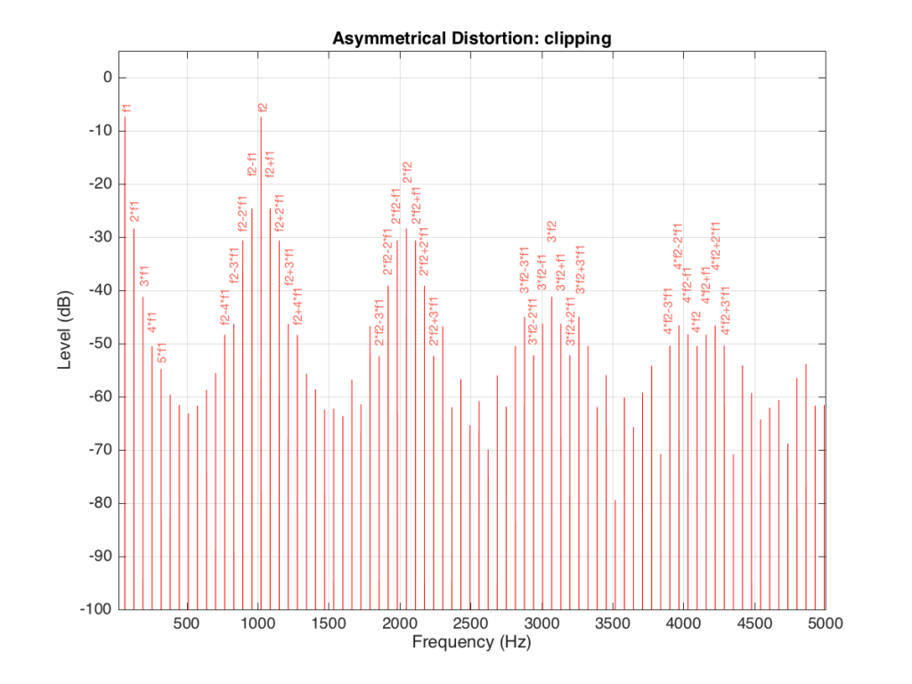
If we were to look at the frequency content of the asymmetrically-distorted signal (shown in Figures 3 and 4), the result would be as is shown in Figure 9.
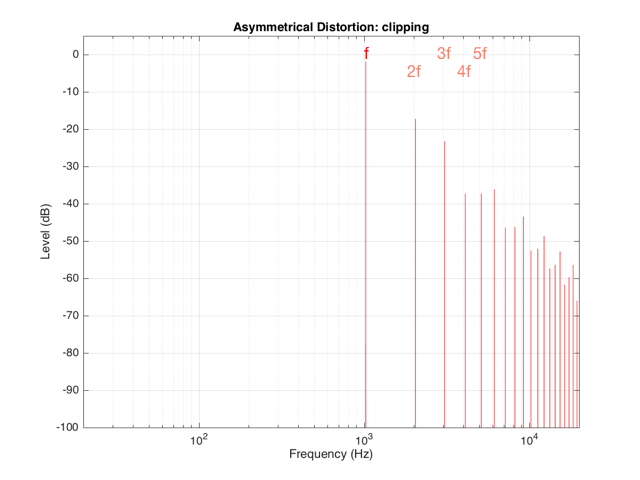
In Figure 9, you can see at least two interesting things:
The first is that the level of the fundamental frequency of “f” (1024 Hz) is higher than it was in Figure 8. This is because we’re letting more of the energy of the original waveform through the distortion (because the negative portion is untouched).
The second thing that you can see in Figure 9 is that both the odd-order and the even-order harmonics are showing up. So, we get energy at 2048 Hz (2*1024), 3072 Hz (3*1024), 4096 Hz (4*1024), 5120 Hz (5*1024), and so on. The presence of the even-order harmonics tells us that either the input signal was asymmetrical (which it wasn’t) or that the distortion applied to it was asymmetrical (which is was) or both.
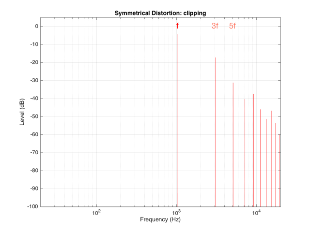
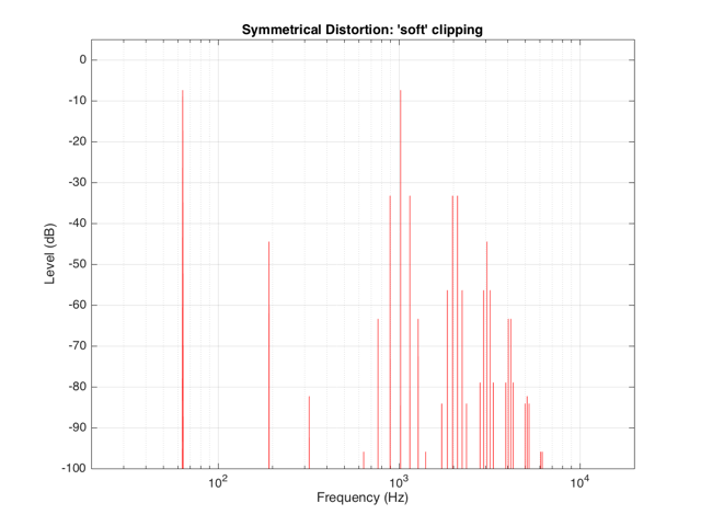
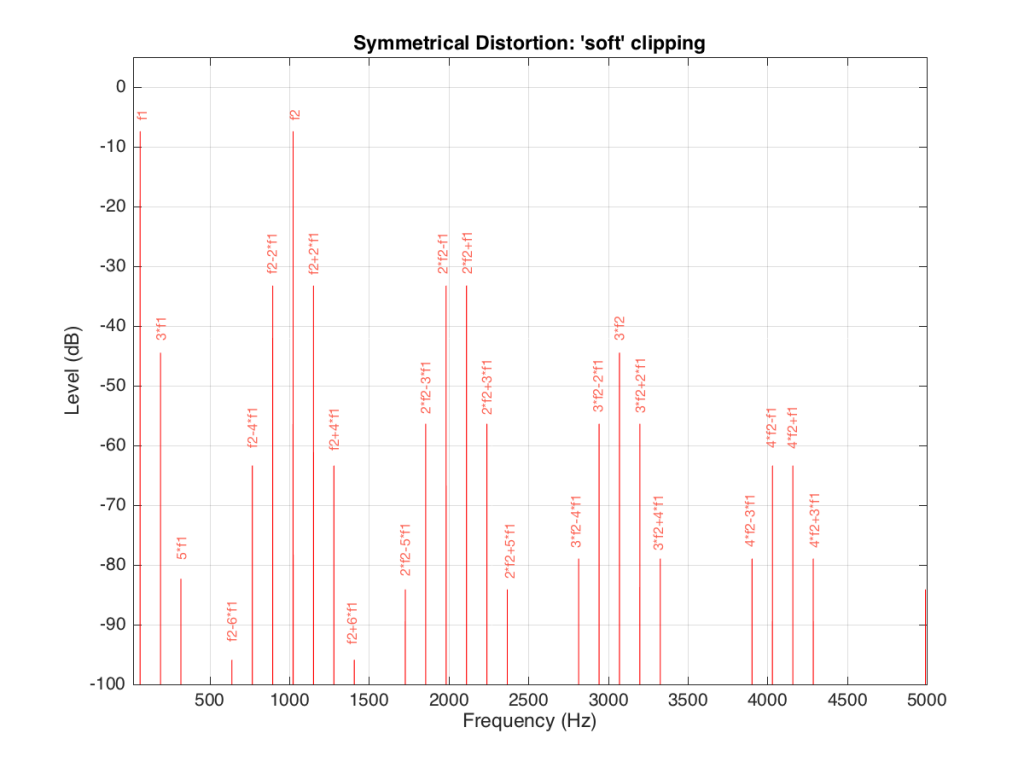
If the distortion we apply to the signal was less abrupt – using the “soft-clipping” function shown in Figure 5 and 6, the result would be different, as is shown in Figure 10.
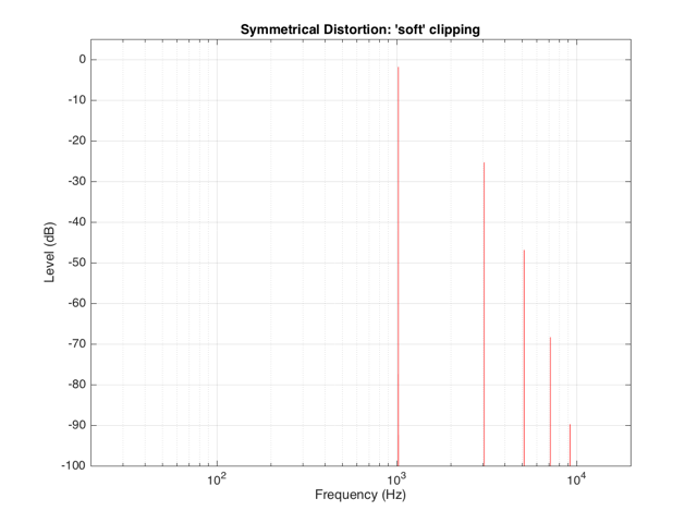
Again, in Figure 10, you can see that only the odd-order harmonics appear as the distortion products, since the distortion we’re applying to the symmetrical signal is symmetrical.
Intermodulation Distortion
So far, we’ve only been looking at the simple case of an input signal with a single frequency. Typically, however, research has shown that most persons listen to more than one frequency simultaneously (acoustical engineers and Stockhausen enthusiasts excepted…). So, let’s look at what happens when we have more than one frequency – say, two frequencies – in our input signal.
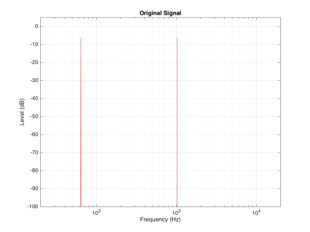
For example, let’s say that we have an input signal, the frequency content of which is shown in Figure 11, consisting of sinusoidal tones at 64 Hz and 1024 Hz. Both sine tones, individually, have a peak level of one-half of the maximum peak of the system. Therefore, they are shown in Figure 11 as having a level of approximately -6 dB each.
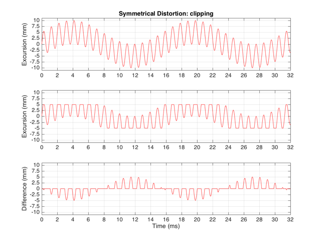
The sum of these two sinusoids will look like the top plot in Figure 12. As you can see there, the signal with the higher frequency is “riding on top of” the signal with the lower frequency. Each frequency, on its own, is pushing and pulling the excursion by ±5 mm. The total result therefore can move from -10 mm to +10 mm, but its instantaneous value is dependent on the overlap of the two signals at any one moment.
If we apply the symmetrical clipping shown in Figure 1 to this signal, the result is as is shown in the middle plot of Figure 12 (with the error shown in the bottom plot). This results in an interesting effect since, although the distortion we’re applying should be symmetrical, the result at any given moment is asymmetrical. This is because the signal itself is asymmetrical with respect to the clipping – the high frequency component alternates between getting clipped on the top and the bottom, depending on where the low frequency component has put it…
We can look at the frequency content of the resulting clipped signal. This is shown in Figure 13.
It’s obvious from the plot in Figure 13 that we have a mess. However, although the mess is rather systematic, it’s difficult to see in that plot. If we plot the same information on a different scale, things get easier to understand. Take a look at Figure 14.
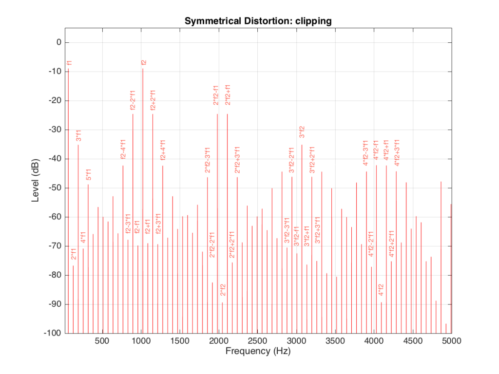
Figure 14 and Figure 13 show exactly the same information with only two differences. The first is that Figure 14 only shows frequencies up to 5 kHz instead of 20 kHz. The second is that the scale of the x-axis of Figure 13 is logarithmic whereas the scale of Figure 14 is linear. This is only a chance in spacing, but it makes things easier to understand.
As you can see in Figure 14, the extra frequencies added to the original signal by the clipping are regularly spaced. This is because the distortion that we have generated (called an intermodulation distortion, since it results from two two signals modulating each other), in the frequency domain, follows a pretty simple mathematical pattern.
Our original two frequencies of 64 Hz (called “f1” on the plot) and 1024 Hz (“f2”) are still present.
In addition, the sum and difference of these two frequencies are also present (f2+f1 = 1088 Hz and f2-f1 = 1018 Hz).
The sum and difference of the harmonic distortion products of the frequencies are also present. For example, 2*f2+f1 = 2*1024+64=2112 Hz, 3*fs-2*f1 = 3*1024-2*64 = 2944 Hz… There are many, many more of these. Take one frequency, multiply it by an integer and then add (or subtract) that from the other frequency multiplied by an integer – whatever the result, that frequency will be there. Don’t worry if your result is negative – that’s also in there (although we’re not going to talk about negative frequencies today – but trust me, they exist…)
If we apply the asymmetrical clipping to the same signal, we (of course) get a different result, but it exhibits the same characteristics, just with different values, as can be seen in Figures 15 and 16.
Wrapping up
It’s important to state once more that none of the plots I’ve shown here are based on any real loudspeaker driver. I’m using simple examples of non-linear distortion just to illustrate the effects on an audio signal. The actual behaviour of an actual loudspeaker driver will be much more complicated than this, but also much more subtle (hopefully – if not, something it probably broken…).
Appendix
As I mentioned at the very beginning of this posting, many of the plots in this article have an intentional error. The reason I wrote this article is to try to give you an intuitive understanding of the results of a problem with the stiffness and Bl curves of a loudspeaker driver with respect to its excursion. This means that my plots of the time domain (such as those in Figure 2) show the excursion of the driver in millimetres with respect to time. I then skip over to a magnitude response plot, pretending that the signal that comes from a driver (a measurement of the air pressure) is identical to the pattern of the driver’s excursion. This is not true. The modulation in air pressure caused by a moving loudspeaker driver are actually in phase with the acceleration of the loudspeaker driver – not its excursion. So, I skipped a step or two. However, since I wasn’t actually showing real responses from real drivers, I didn’t feel too guilty about this. Just be warned that, if you’re really digging into this, you should not directly jump from loudspeaker driver excursion to a plot of the sound pressure.
Vinyl outsells YouTube

B&O Tech: Headphone signal flows
#54 in a series of articles about the technology behind Bang & Olufsen products
Someone recently asked a question on this posting regarding headphone loudness. Specifically, the question was:
“There is still a big volume difference between H8 on Bluetooth and cable. Why is that?”
I thought that this would make a good topic for a whole posting, rather than just a quick answer to a comment – so here goes…
Introduction – the building blocks
To begin, let’s take a quick look at all the blocks that we’re going to assemble in a chain later. It’s relatively important to understand one or two small details about each block.
Two start:
- I’ve used red lines for digital signals and blue lines for analogue signals. I’ve assumed that the digital signal contains 2 audio channels, and that the analogue connections are one channel each.
- My signal flow goes from left to right
- I use the word “telephone” not because I’m old-fashioned (although I am that…) but because if I say “phone”, I could be mistaken for someone talking about headphones. However, the source does not have to be a telephone, it could be anything that fits the descriptions below.
- The blocks in my signal flows should be taken as basic examples. I have not reverse-engineered a particular telephone or computer or pair of headphones. I’m just describing basic concepts here…

Figure 1, above, shows a 2-channel audio DAC – a Digital to Analogue Converter. This is a device (these days, it’s usually just a chip) that receives a 2-channel digital audio signal as a stream of bits at its input and outputs an analogue signal that is essentially a voltage that varies appropriately over time.
One important thing to remember here is that different DAC’s have different output levels. So, if you send a Full Scale sine wave (say, a 997 Hz, 0 dB FS) into the input of one DAC, you might get 1 V RMS out. If you sent exactly the same input into another DAC (meaning another brand or model) you might get 2 V RMS out.
You’ll find a DAC, for example, inside your telephone, since the data inside it (your MP3 and .wav files) have to be converted to an analogue signal at some point in the chain in order to move the drivers in a pair of headphones connected to the minijack output.

Figure 2, above, shows a 2-channel ADC – and Analogue to Digital Converter. This does the opposite of a DAC – it receives two analogue audio channels, each one a voltage that varies in time, and converts that to a 2-channel digital representation at its output.
One important thing to remember here is the sensitivity of the input of the ADC. When you make (or use) an ADC, one way to help maximise your signal-to-noise ratio (how much louder the music is than the background noise of the device itself) is to make the highest analogue signal level produce a full-scale representation at the digital output. However, different ADC’s have different sensitivities. One ADC might be designed so that 2.0 V RMS signal at its input results in a 0 dB FS (full scale) output. Another ADC might be designed so that a 0.5 V RMS signal at its input results in a 0 dB FS output. If you send 0.5 V RMS to the first ADC (expecting a max of 2 V RMS) then you’ll get an output of approximately -12 dB FS. If you send 2 V RMS to the second ADC (which expects a maximum of only 0.5 V RMS) then you’ll clip the signal.

Figure 3, above, shows a Digital Signal Processor or DSP. This is just the component that does the calculations on the audio signals. The word “calculations” here can mean a lot of different things: it might be a simple volume control, it could be the filtering for a bass or treble control, or, in an extreme case, it might be doing fancy things like compression, upmixing, bass management, processing of headphone signals to make things sound like they’re outside your head, dynamic control of signals to make sure you don’t melt your woofers – anything…

Figure 4, above, shows a two-channel analogue amplifier block. This is typically somewhere in the audio chain because the output of the DAC that is used to drive the headphones either can’t provide a high-enough voltage or current (or both) to drive the headphones. So, the amplifier is there to make the voltage higher, or to be able to provide enough current to the headphones to make them loud enough so that the kids don’t complain.

The final building block in the chain is the headphone driver itself. In most pairs of headphones, this is comprised of a circular-shaped magnet with a coil of wire inside it. The coil is glued to a diaphragm that can move like the skin of a drum. Sending electrical current back and forth through the coil causes it to move back and forth which pushes and pulls the diaphragm. That, in turn, pushes and pulls the air molecules next to it, generating high and low pressure waves that move outwards from the front of the diaphragm and towards your eardrum. If you’d like to know more about this basic concept – this posting will help.
One important thing to note about a headphone driver is its sensitivity. This is a measure of how loud the output sound is for a given input voltage. The persons who designed the headphone driver’s components determine this sensitivity by changing things like the strength of the magnet, the length of the coil of wire, the weight of the moving parts, resonant chambers around it, and other things. However, the basic point here is that different drivers will have different loudnesses at different frequencies for the same input voltage.
Now that we have all of those building blocks, let’s see how they’re put together so that you can listen to Foo Fighters on your phone.
Version 1: The good-old days
In the olden days, you had a pair of headphones with a wire hanging out of one or both sides and you plugged that wire into the headphone jack of a telephone or computer or something else. We’ll stick with the example of a telephone to keep things consistent.
Figure 6, below, shows an example of the path the audio signal takes from being a MP3 or .wav (or something else) file on your phone to the sound getting into your ears.
The file is read and then decoded into something called a “PCM” signal (Pulse Code Modulation – it doesn’t matter what this is for the purposes of this posting). So, we get to point “A” in the chain and we have audio. In some cases, the decoder doesn’t have to do anything (for example, if you use uncompressed PCM audio like a .wav file) – in other cases (like MP3) the decoder has to convert a stream of data into something that can be understood as an audio signal by the DSP. In essence, the decoder is just a kind of universal translator, because the DSP only speaks one language.
The signal then goes through the DSP, which, in a very simple case is just the volume control. For example, if you want the signal to have half the level, then the DSP just multiplies the incoming numbers (the audio signal) by 0.5 and spits them out again. (No, I’m not going to talk about dither today.) So, that gets us to point “B” in the chain. Note that, if your volume is set to maximum and you aren’t doing anything like changing the bass or treble or anything else – it could be that the DSP just spits out what it’s fed (by multiplying all incoming values by 1.0).
Now, the signal has to be converted to analogue using the DAC. Remember (from above) that the actual voltage at its output (at point “C”) is dependent on the brand and model of DAC we’re talking about. However, that will probably change anyway, since the signal is fed through the amplifiers which output to the minijack connector at point “D”.
Assuming that they’ve set the DSP so that output=input for now, then the voltage level at the output (at “D”) is determined by the telephone’s manufacturer by looking at the DAC’s output voltage and setting the gain of the amplifiers to produce a desired output.
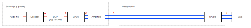
Then, you plug a pair of headphones into the minijack. The headphone drivers have a sensitivity (a measure of the amount of sound output for a given voltage/current input) that will have an influence on the output level at your eardrum. The more sensitive the drivers to the electrical input, the louder the output. However, since, in this case, we’re talking about an electromechanical system, it will not change its behaviour (much) for different sources. So, if you plug a pair of headphones into a minijack that is supplying 2.0 V RMS, you’ll get 4 times as much sound output as when you plug them into a minijack that is supplying 0.5 V RMS.
This is important, since different devices have VERY different output levels – and therefore the headphones will behave accordingly. I regularly measure the maximum output level of phones, computers, CD players, preamps and so on – just to get an idea of what’s on the market. I’ve seen maximum output levels on a headphone jack as low as 0.28 V RMS (on an Apple iPod Nano Gen4) and as high as 8.11 V RMS (on a Behringer Powerplay Pro-8 headphone distribution amp). This is a very big difference (29 dB, which also happens to be 29 times…).
Version 2: The more-recent past
So, you’ve recently gone out and bought yourself a newfangled pair of noise-cancelling headphones, but you’re a fan of wires, so you keep them plugged into the minijack output of your telephone. Ignoring the noise-cancelling portion, the signal flow that the audio follows, going from a file in the memory to some sound in your ears is probably something like that shown in Figure 7.
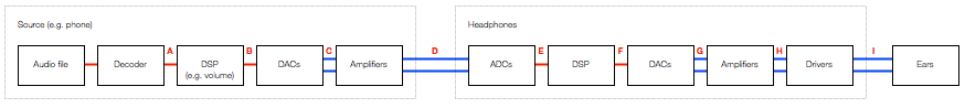
As you can see by comparing Figures 7 and 6, the two systems are probably identical until you hit the input of the headphones. So, everything that I said in the previous section up to the output of the telephone’s amplifiers is the same. However, things change when we hit the input of the headphones.
The input of the headphones is an analogue to digital converter. As we saw above, the designer of the ADC (and its analogue input stages) had to make a decision about its sensitivity – the relationship between the voltage of the analogue signal at its input and the level of the digital signal at its output. In this case, the designer of the headphones had to make an assumption/decision about the maximum voltage output of the source device.
Now we’re at point “E” in the signal chain. Let’s say that there is no DSP in the headphones – no tuning, no volume – nothing. So, the signal that comes out of the ADC is sent, bit for bit, to its DAC. Just like the DAC in the source, the headphone’s DAC has some analogue output level for its digital input level. Note that there is no reason for the analogue signal level of the headphones’ input to be identical to the analogue output level of the DAC or the analogue output level of the amplifiers. The only reason a manufacturer might want to try to match the level between the analogue input and the amplifier output is if the headphones work when they’re turned off – thus connecting the source’s amplifier directly to the headphone drivers (just like in Figure 6). This was one of the goals with the BeoPlay H8 – to ensure that if your batteries die, the overall level of the headphones didn’t change considerably.
However, some headphones don’t bother with this alignment because when the batteries die, or you turn them off, they don’t work – there’s no bypass…
Version 3: Look ma! No wires!
These days, many people use Bluetooth to connect wirelessly from the source to the headphones. This means that some components in the chain are omitted (like the DAC’s in the source and the ADC in the headphones) and others are inserted (in Figures 8 and 9, the Bluetooth Transmitter and Receiver).
Note that, to keep things simple, I have not included the encoder and the decoder for the Bluetooth transmission in the chain. Depending mainly on your source’s capabilities, the audio signal will probably be encoded into one of the varieties of an SBC, an AAC, or an aptX codec before transmitting. It’s then decoded back to PCM after receiving. In theory, the output of the decoder has the same level as the input of the encoder, so I’ve left it out of this discussion. I won’t discuss either CODEC’s implications on audio quality in this posting.
Taking a look at Figure 8 or 9 and you’ll see that, in theory, the level of the digital audio signal inside the source is identical to that inside the headphones – or, at least, it can be.
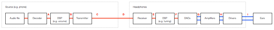
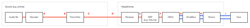
This means that the potentially incorrect assumptions made by the headphone manufacturer about the analogue output levels of the source can be avoided. However, it also means that, if you have a pair of headphones like the BeoPlay H7 or H8 that can be used either via an analogue or a Bluetooth connection then there will, in many cases, be a difference in level when switching between the two signal paths.
For example…
Let’s take a simple case. We’ll build a pair of headphones that can be used in two ways. The first is using an analogue input that is processed through the headphone’s internal DSP (just as is shown in Figure 6). We’ll build the headphones so that they can be used with a 2.0 V RMS output – therefore we’ll set the input sensitivity so that a 2.0 V RMS signal will result in a 0 dB FS signal internally.
We then connect the headphones to an Apple MacBook Pro’s headphone output, we play a signal with a level of 0 dB FS, and we turn up the volume to maximum. This will result in an analogue violate level of 2.085 V RMS coming from the computer’s headphone output.
Now we’ll use the same headphones and connect them to an Apple iPhone 4s which has a maximum analogue output level of 0.92 V RMS. This is less than half the level of the MacBook Pro’s output. So, if we set the volume to maximum on the iPhone and play exactly the same file as on the MacBook Pro, the headphones will have half the output level.
A second way to connect the headphones is via Bluetooth using the signal flow shown in Figure 8. Now, if we use Bluetooth to connect the headphones to the MacBook Pro with its volume set to maximum, a 0 dB FS signal inside the computer results in a 0 dB FS signal inside the headphones.
If we connect the headphones to the iPhone 4s via Bluetooth and play the same file at maximum volume, we’ll get the same output as we did with the MacBook Pro. This is because the 0 dB FS signal inside the phone is also producing a 0 dB FS signal in the headphones.
So, if you’re on the computer, switching from a Bluetooth connection to an analogue wired connection using the same volume settings will result in the same output level from the headphones (because the headphones are designed for a max 2 V RMS analogue signal). However, if you’re using the telephone, switching from a Bluetooth connection to an analogue wired connection will results in a drop in the output level by more than 6 dB (because the telephone’s maximum output level is less than 1 V RMS).
Wrapping up
So, the answer to the initial question is that there’s a difference between the output of the H8 headphones when switching between Bluetooth and the cable because the output level of the source that you’re using is different from what was anticipated by the engineers who designed the input stage of the headphones. This is likely because the input stage of the headphones was designed to be compatible with a device with a higher maximum output level than the one you’re using.