A fourth-order Linkwitz-Riley crossover is made using the same filters in the 2nd-order Butterworth crossover described in the previous posting. The difference in implementation is that you use two second-order filters in series. Again, all filters have the same cutoff frequency and, if you’re implementing them with biquads, the Q of all of them is 1/sqrt(2).
Figure 3.1
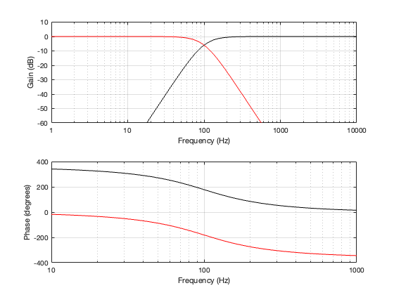
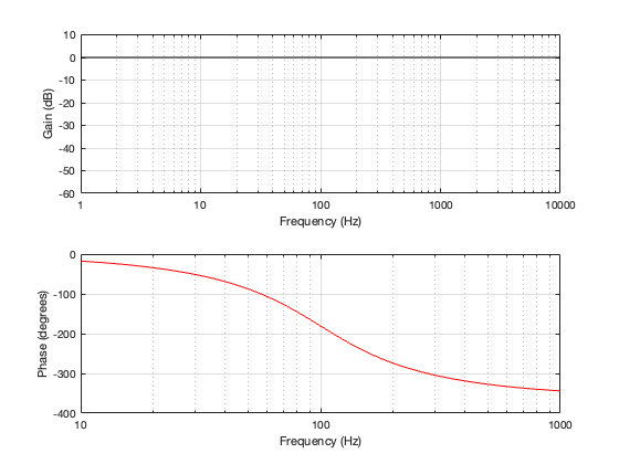
Since we have two high pass filters in series, then the total result is -6 dB at the cutoff frequency (since each of the two filters attenuates by 3 dB) and the slope of the filter is 24 dB per octave. This results in the magnitude and phase responses shown below in Figure 3.2.
Figure 3.2
One important thing to notice now is that the phase responses of the two filters are 360º apart at all frequencies. This is different from the second-order Butterworth crossover, in which the two outputs are 180º apart. So we won’t need to flip the polarity of anything to compensate for the phase difference.
As in the previous posting, Let’s look at the signals that get through the crossover, and the total summed output for three input frequencies. This is shown in Figure 3.3, 3.4, and 3.5.
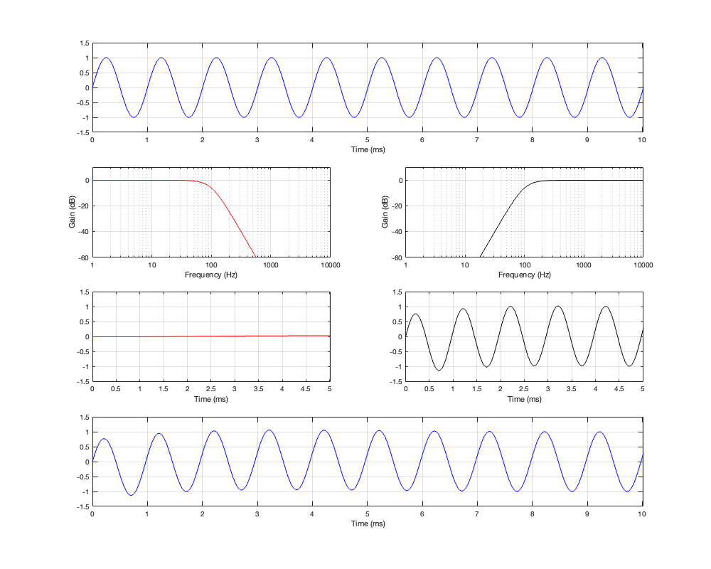
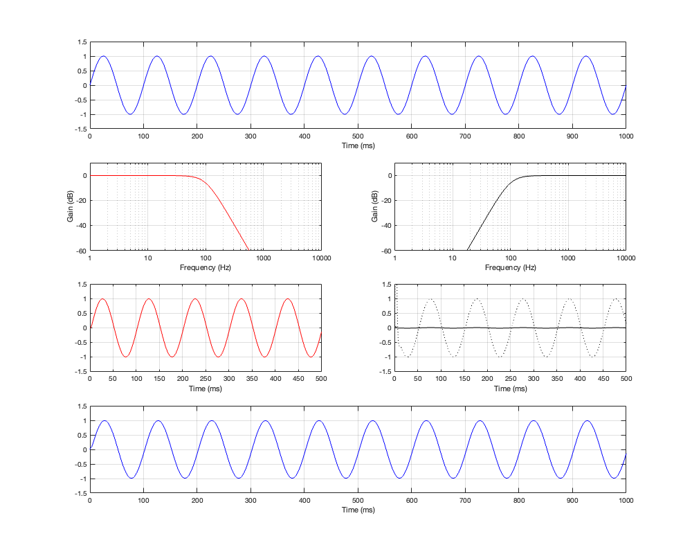
Figure 3.3: Row 1: the input (1 kHz sine wave). Row 2: the magnitude responses of the two filters. Row 3: the outputs of the individual filters. Row 4: the summed output
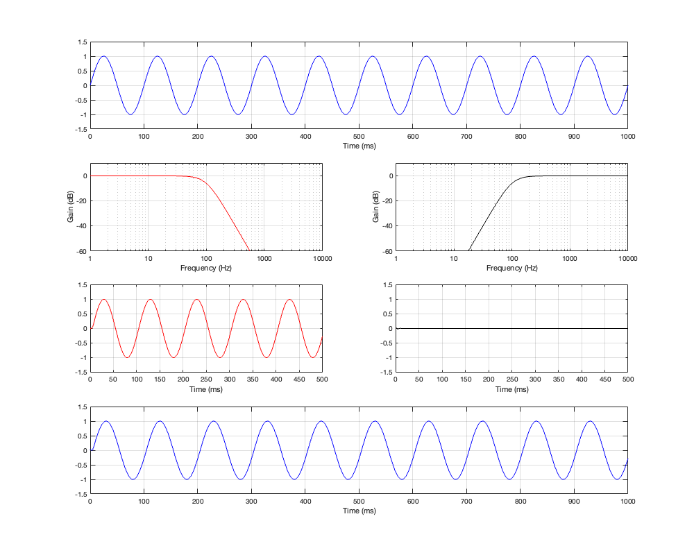
Figure 3.4: Row 1: the input (10 Hz sine wave). Row 2: the magnitude responses of the two filters. Row 3: the outputs of the individual filters. Row 4: the summed output
Figure 3.5: Row 1: the input (100 Hz sine wave). Row 2: the magnitude responses of the two filters. Row 3: the outputs of the individual filters. Row 4: the summed output
If you take a look at Figures 3.3 and 3.4 it appears that the total summed output of the crossover is in phase with the input at very low and very high frequencies. However, this is actually misleading. Take a look at Figure 3.5 and you’ll see that, when the input signal is the same frequency as the crossover frequency, the summed output is shifted by 180º relative to the input signal.
Figure 3.6
If we compare the summed output to the input, they are in-phase at very low frequencies. As the frequency increases, the phase of the summed output of the crossover gets later and later, passing 180º at the crossover frequency and approaching a shift of 360º in the high frequencies.
In other words, a 4th-order Linkwitz-Riley crossover by itself, when you sum the outputs of the filters as shown in Figure 3.1, has the same response as a 4th-order minimum phase allpass filter.
One extra thing to notice is that, since the high-pass and low-pass paths are 360º apart, and (partly) since they’re -6 dB at the crossover frequency, the magnitude response of the summed total is flat.
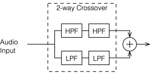
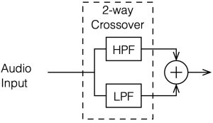
One way to look at the behaviour of a signal when it’s sent through a crossover is to pretend that the loudspeaker isn’t part of the system. Once-upon-a-time, I probably would have phrased this differently and said something like “pretend that the loudspeaker is perfect”, but, now that I’m older, my opinions about the definition of “perfect” have changed.
So, we’ll take a signal, send it to a two-way crossover of some kind, and then just add the two signals back together. This shows us one view of the behaviour of the crossover, which is good enough to deal with the basics for now. In a later posting in this series, we’ll look at a more multi-dimensional and therefore realistic view of what’s happening.
Figure 2.1
The block diagram above shows the signal flow that I used for all of the following plots in this posting.
Butterworth, 2nd-order (12 db/octave)
Although the block diagram above shows that we have a high-pass and a low-pass filter to separate the signal into two frequency bands, there are a lot of details missing about the specific characteristics of those filters. There are many ways to make a high-pass filter, for example…
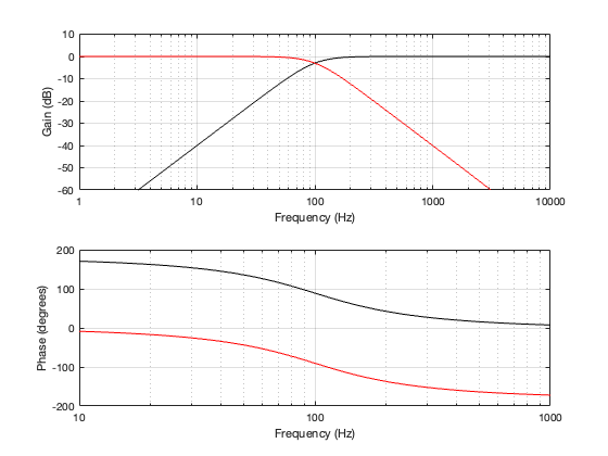
One common crossover type uses 2nd-order Butterworth filters, both with the same cutoff frequency. One way to implement these are to use biquads to make low-pass and high-pass filters with Q = 1/sqrt(2).
Fig. 2.2: The individual magnitude and phase responses of the low-pass (in red) and high-pass (in black)
Before we look at the output of the entire crossover after the two signals have been summed, let’s talk about the red and the black curves in the plots above.
The magnitude responses should not come as a surprise. The fact that I’m using 2nd-order filters means that the slope of the attenuation will be 12 dB per octave (or 40 dB per decade) once you get far enough away from the cutoff frequency. The fact that they also have a Q of 1/sqrt(2) (approximately 0.707) means that they will attenuate the signal by 3 dB at the cutoff frequency, and that there is no “bump” in the slope of the magnitude response.
However, the phase responses might be a little confusing. Let’s take those separately:
For the low-pass filter (the black line), you can see that in the high-frequency band, where the magnitude response is a flat line at 0 dB (which means that the level of the output level is equal to the level of the input), the phase shift is 0º.
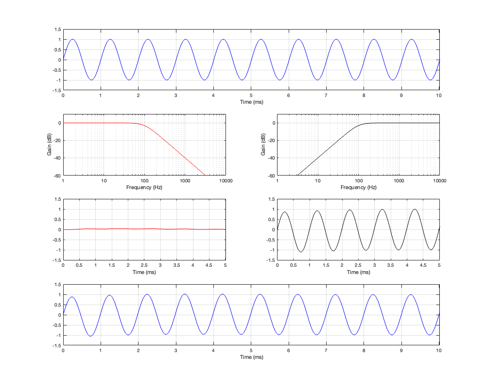
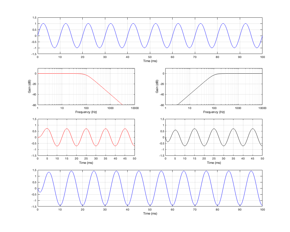
Another way to look at this is to put a sine wave into the system and see what comes out, as shown in Figure 2.3 below. The top plot shows the input to the two filters. Since this sine wave has a period of 1 ms, then it’s a 1000 Hz tone.
The second row of plots shows the magnitude responses of the low-pass filter (in red, on the left) and the high-pass filter (in black, on the right). Notice the levels of these two curves at a frequency of 1000 Hz.
The third row of plots shows the actual outputs of the two filters. For now, we’ll only look at the output of the high-pass filter on the right. There are three things to notice about this plot:
After about 1 ms, the amplitude of this sine tone is the same as the one in the top plot.
The phase of this sine tone is the same as the one in the top plot. In other words (for example), they both pass the 0 line, heading positive at Time = 1 ms.
The start of the sine wave is a little weird. Notice that the positive peak is lower than expected and first negative trough is BELOW the maximum-negative amplitude. (it’s below a value of -1). We’ll ignore this for now, and come back to it later.
The fourth row shows the output of the two filters when they have been added together. Notice here that the output is almost identical to the input because it’s essentially just the contribution of the high-pass filter. The low-pass filter has so little output that it’s practically irrelevant.
Figure 2.3: Row 1: the input (1 kHz sine wave). Row 2: the magnitude responses of the two filters. Row 3: the outputs of the individual filters. Row 4: the summed output
Let’s now look a what happens if we put in a low-frequency sine wave instead. This is shown in Figure 2.4.
Figure 2.4 Row 1: the input (10 Hz sine wave). Row 2: the magnitude responses of the two filters. Row 3: the outputs of the individual filters. (the dotted line shows the signal with its amplitude multiplied by 10 to “zoom in” on it) Row 4: the summed output
Notice now that the time scale is 100 times longer. The sine wave now has a period of 100 ms, so it’s a 10 Hz sine wave.
We’ll focus on the third row of plots again, still looking only at the output of the high-pass filter on the right. There are three things to notice about this plot:
After about 100 ms, the amplitude of this sine tone (the solid black line) is MUCH lower than the amplitude of the input. The dotted line is a “magnified” version of the same signal so that we can see it for the phase comparison.
The phase of this sine tone is the shifted by 180º relative to the top plot. In other words (for example), at Time = 200 ms they both pass the 0 line, but this signal is going negative when the input is going positive.
The start of the sine wave is a also weird, but differently so; with that spike at the beginning and the weird wiggle in the curve before it settles down. We’ll ignore this for now, and come back to it later.
If you go back and look at the low-pass filter’s output, then you’ll see basically the same behaviour, but for the opposite frequency.
And, again, the output is almost identical to the input because it’s essentially just the contribution of the low-pass filter. The high-pass filter has so little output that it’s practically irrelevant.
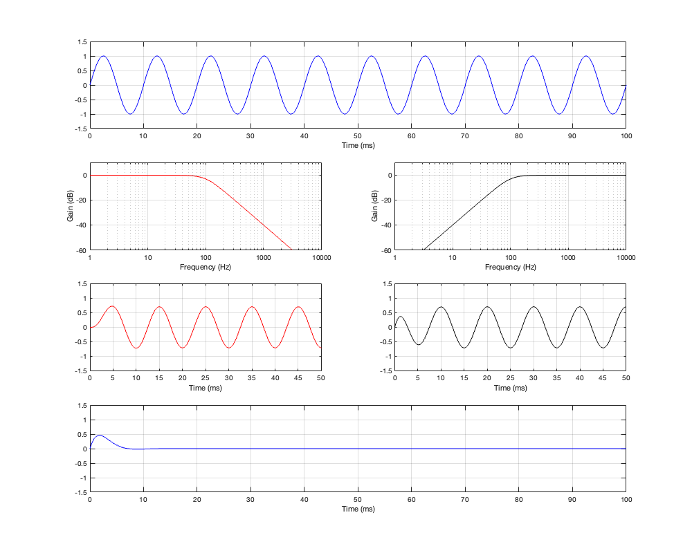
Now let’s look at what happens when the frequency of the input signal is on the cutoff frequency of the two filters – in other words, the crossover frequency.
Figure 2.5: Row 1: the input (100 Hz sine wave). Row 2: the magnitude responses of the two filters. Row 3: the outputs of the individual filters. Row 4: the summed output
Now the sine wave has a period of 10 ms, so its frequency is 100 Hz.
Take a look at the third row of plots at Time = 10 ms.
The first thing to do is to compare the outputs of the two filters. The output of the low-pass filter on the left is negative, whereas the output of the high-pass filter on the right is positive. The outputs of the two filters are 180º out of phase with each other. This can also be seen in the plot back in Figure 2.2, where it’s shown that the difference between the red and the black phase response plots is 180º at all frequencies.
This is also why., once everything settles down, the sum of the two filters (the blue line on the bottom) is silence. The two signals have equal amplitude, and are 180º out of phase, so they cancel each other out.
Now compare those signal plots in the third row in Figure 2.5 to the input signal shown in the top plot. If you look at Time = 10 ms again (for example), you can see that the output of the low-pass filter is 90º behind the input. However, the output of the high-pass filter is early 90º ahead of the input.
The fact that the phase of the output of the high-pass filter is ahead of its own input confuses many people, however, don’t panic. This does not mean that the output is ahead of the input in TIME. The high-pass filter cannot see into the future. The only reason its output can have a phase that precedes the phase of its input is if the sine wave has been playing for a long time (and, in this case a “long” time can be measured in milliseconds…).
This confusion is the result of two things:
People are typically taught the concept of phase as it relates to time. However, if you’re talking about a sine wave, then you are implying infinite time. in order for a signal to be a REAL sine wave, it must have always been playing and it must never stop. If it started or stopped, then there are other frequencies present, and so it’s not a theoretically-perfect sine wave.
We use the words “ahead” and “behind” or “earlier” and “later” to describe the phase relationships, and these words typically imply a time relationship.
Maybe a rough analogy that can help is to walk next to a friend, at the same speed, but do not synchronise your steps. You will both arrive at the same place at the same time, but at two different moments in the cycles of your footsteps.
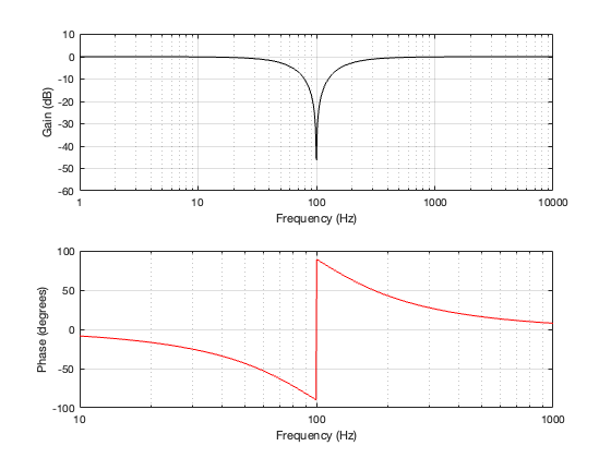
Of course, if you make a crossover like this, it won’t work very well, since you get that cancellation at the crossover frequency when the two filters outputs are added together. If we plot the summed response’s magnitude and phase characteristics, they look like the plots shown in Figure 2.6.
Figure 2.6: the magnitude and phase responses of the total shown in Figure 2.5.
As you can see there, there is complete cancellation at the crossover frequency, and the phase response flips across that notch.
So, the solution with a 2nd-order Butterworth crossover is to assume that people won’t notice if you invert the polarity of the high-pass filter’s output. This is a good assumption that I will not argue with at all.
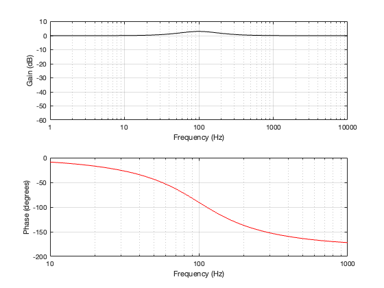
This polarity inversion “undoes” the 180º phase difference of the two filters seen in Figure 2.2, and the summed result is shown below in Figure 2.7 and 2.8.
Figure 2.7: the magnitude and phase responses of the total shown in Figure 2.8, which is the same as Figure 2.5 after the polarity of the HPF’s output has been inverted.
Figure 2.8: Row 1: the input (100 Hz sine wave). Row 2: the magnitude responses of the two filters. Row 3: the outputs of the individual filters. (Note that the polarity of the HPF’s output has been inverted) Row 4: the summed output
Now the outputs of the two filters appear to be in phase with each other. They are still 90º out of phase with the input, which means that their summed outputs are also 90º out of phase with the input. This can be seen in the bottom plots of Figure 2.7 and 2.8.
You’ll also notice that there is a 3 dB bump at the crossover frequency. This is because, at their cutoff frequencies, both filters attenuate by 3 dB (a linear gain of 0.707). When those two signals of equal amplitude and matching phase are added together, you get a magnitude that is 6 dB higher (or a linear gain of 1.41). We’ll talk about this later when we start looking at the real world.
Finally, take a look at the bottom plot in Figure 2.7. You can see there that the summed outputs of the two filters result in a phase shift that increases with frequency. In fact, when we look at a 2nd-order Butterworth crossover like this, without all the real-world implications of loudspeaker drivers that have their own characteristics and are separated in space, it can be seen that it acts as a 2nd-order minimum-phase allpass filter. This isn’t necessarily a bad thing, so don’t jump to conclusions this early…
We are STILL not going to talk about that weirdness at the beginning of the signal after it’s been filtered. That will come later.
A crossover is a set of filters that take an audio signal and separate it into different frequency portions or “bands”.
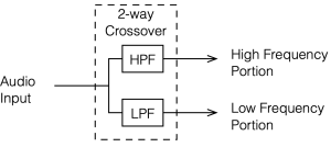
For example, possibly the simplest type of crossover will accept an audio signal at its input, and divide it into the high frequency and the low frequency components, and output those two signals separately. In this simple case, the filtering would be done with
a high-pass filter (which allows the high frequency bands to pass through and increasingly attenuates the signal level as you go lower in frequency), and
a low-pass filter (which allows the low frequency bands to pass through and increasingly attenuates the signal level as you go higher in frequency).
This would be called a “Two-way crossover” since it has two outputs.
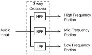
Crossovers with more outputs (e.g. Three- or Four-way crossovers) are also common. These would probably use one or more band-pass filters to separate the mid-band frequencies.
Why do we need crossovers?
In order to understand why we might need a crossover in a loudspeaker, we need to talk about loudspeaker drivers, what they do well, and what they do poorly.
It’s nice to think of a loudspeaker driver like a woofer or a tweeter as a rigid piston that moves in and out of an enclosure, pushing and pulling air particles to make pressure waves that radiate outwards into the listening room. In many aspects, this simplified model works well, but it leaves out a lot of important information that can’t be ignored. If we could ignore the details, then we could just send the entire frequency range into a single loudspeaker driver and not worry about it. However, reality has a habit of making things difficult.
For example, the moving parts of a loudspeaker driver have a mass that is dependent on how big it is and what it’s made of. The loudspeaker’s motor (probably a coil of wire living inside a magnetic field) does the work of pushing and pulling that mass back and forth. However, if the frequency that you’re trying to produce is very high, then you’re trying to move that mass very quickly, and inertia will work against you. In fact, if you try to move a heavy driver (like a woofer) a lot at a very high frequency, you will probably wind up just burning out the motor (which means that you’ve melted the wire in the coil) because it’s working so hard.
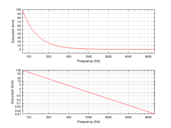
Another problem is that of loudspeaker excursion, how far it moves in and out in order to make sound. Although it’s not commonly known, the acoustic output level of a loudspeaker driver is proportional to its acceleration (which is a measure of its change in velocity over time, which are dependent on its excursion and the frequency it’s producing). The short version of this relationship is that, if you want to maintain the same output level, and you double the frequency, the driver’s excursion should reduce to 1/4. In other words, if you’re playing a signal at 1000 Hz, and the driver is moving in and out by ±1 mm, if you change to 2000 Hz, the driver should move in and out by ±0.25 mm. Conversely, if you halve the frequency to 500 Hz, you have to move the driver in and out with an excursion of ±4 mm. If you go to 1/10 of the frequency, the excursion has to be 100x the original value. For normal loudspeakers, this kind of range of movement is impractical, if not impossible.
Note that both of these plots show the same thing. The only difference is the scaling of the Y-axis.
One last example is that of directivity. The width of the beam of sound that is radiated by a loudspeaker driver is heavily dependent on the relationship between its size (assuming that it’s a circular driver, then its diameter) and the wavelength (in air) of the signal that it’s producing. If the wavelength of the signal is big compared to the diameter of the driver, then the sound will be radiated roughly equally in all directions. However, if the wavelength of the signal is similar to the diameter of the driver, then it will emit more of a “beam” of sound that is increasingly narrow as the frequency increases.
So, if you want to keep from melting your loudspeaker driver’s voice coil you’ll have to increasingly attenuate its input level at higher frequencies. If you want to avoid trying to push and pull your tweeter too far in and out, you’ll have to increasingly attenuate its input level at lower frequencies. And if you’re worried about the directivity of your loudspeaker, you’ll have to use more than one loudspeaker driver and divide up the signal into different frequency bands for the various outputs.
In passive crossovers, many are phase incoherent, meaning that the phase shift of one frequency will be different than another frequency. Do you agree? Am curious how this is dealt with in the active crossover’s of B&O products?
At first, I debated just sending a quick email back with a short answer saying something pithy. But while I was thinking about what to write, I realised that:
This is actually a really good question / topic
I haven’t posted anything about crossovers in a long time
I’ve learned a lot about crossovers since the last time I did post something
I still have a LOT more to learn about crossovers.
As a result, this will be the first in what I expect to be a long series of postings about loudspeaker crossovers, starting with basic questions like
Why do we use them?
What do we think they do?
What do they really do? and
How are the ones we implement these days different from the ones you read about in old textbooks?
As usual, I’ll probably get distracted and wind up going down more than one rabbit hole along the way… But that’s one of the reasons why I’m doing this – to find out where I wind up, and hopefully to meet some new rabbits along the way.
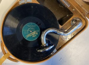
Once-upon-a-time, before there was streaming, and SACDs, and CDs, and vinyl records, and 78 RPM shellac disks, there were cylinders.
I’m part-way through a three-part lecture at the local museum on the history of recorded sound. A portion of Part 1 was to talk about cylinders, and I was lucky enough to meet a local collector who owned a number of cylinder players, one of which he loaned to me for a demonstration.
After some back-and-forth, he agreed to sell me the player to add to my collection. And, after a little (but very little) internal debate, I decided to do a partial restoration as a little weekend project.
The player is about 120 years old, so there’s plenty of dirt and oxide on it. My goal was not to make it as-good-as-new, rather to just clean it up a little.
The easiest part was polishing the screw heads. I made a small brass handle to make this easier…
Before and after polishing one of the steel rods that are used to support the sled.
The various parts of the speed governor, dismantled, and ready for polishing.
Back together again after polishing
The cast-iron base before stripping the paint.
The end support for the two arms and the threaded rod that moves the sled in sync with the groove on the cylinder, before stripping. Note the professional decorative artwork…
The support arm for the speed governor before stripping.
The sled before polishing.
Most of the steel and brass bits and pieces after polishing. The belt on the top left of the photo is made of thin leather.
The original wooden knob for the brake cracked sometime in the past 120 years. So, I made a new one from Cumberland ebonite. I didn’t feel too bad about using this instead of wood, since ebonite was a common material for such things back in those days. The reason I have it on hand is for making fountain pens and replacement parts in restorations.
The last part of the restoration was to hammer and rub out the dents in the bell, and to spend an hour or two sanding the surface with 800-grit paper, and then polishing on a wheel.
After everything went back together, the only thing left to do was to make a wooden base so that the cast iron won’t scratch anything. Rather than try to re-create the original base and cover, I just made a simple one from teak.
The player is NOT sitting on an anti-gravity device. It’s floating above the concrete because it’s sitting on a piece of wood to keep the sand off it before bringing it inside. Note that equally-amateurish decorative paint job on the end piece. I debated making a computer-generated stencil and spray-painting a “perfect” decoration, but I chose to do this instead, in keeping with the original.
“How does it sound?” you ask. I did this recording before the restoration, but you can decide for yourself. Note that, back then, the player still wasn’t mine, and I was hesitant to wind it up enough to play a full two minutes… Hence the rescue mission half-way through.
Now I have to go find some more cylinders. That one is the only one I have, and I’m getting a little tired of “In the Wildwood Where the Bluebells Grew”…
The June, 1968 issue of Wireless World magazine includes an article by R.T. Lovelock called “Loudness Control for a Stereo System”. This article partly addresses the issue of resistance behaviour one or more channels of a variable resistor. However, it also includes the following statement:
It is well known that the sensitivity of the ear does not vary in a linear manner over the whole of the frequency range. The difference in levels between the threshold of audibility and that of pain is much less at very low and very high frequencies than it is in the middle of the audio spectrum. If the frequency response is adjusted to sound correct when the reproduction level is high, it will sound thin and attenuated when the level is turned down to a soft effect. Since some people desire a high level, while others cannot endure it, if the response is maintained constant while the level is altered, the reproduction will be correct at only one of the many preferred levels. If quality is to be maintained at all levels it will be necessary to readjust the tone controls for each setting of the gain control
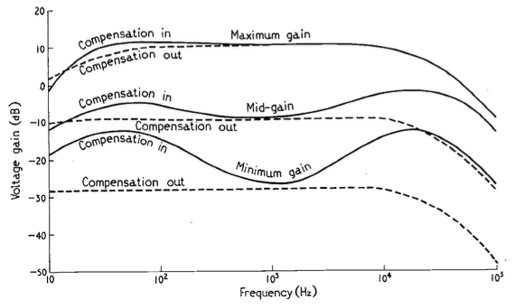
The article includes a circuit diagram that can be used to introduce a low- and high-frequency boost at lower settings of the volume control, with the following example responses:
These days, almost all audio devices include some version of this kind of variable magnitude response, dependent on volume. However, in 1968, this was a rather new idea that generated some debate.
In the following month’s issue The Letters to the Editor include a rather angry letter from John Crabbe (Editor of Hi-Fi News) where he says
Mr. Lovelock’s article in your June issue raises an old bogey which I naively thought had been buried by most British engineers many years ago. I refer, not to the author’s excellent and useful thesis on achieving an accurate gain control law, but to the notion that our hearing system’s non-linear loudness / frequency behaviour justifies an interference with response when reproducing music at various levels.
Of course, we all know about Fletcher-Munson and Robinson-Dadson, etc, and it is true that l.f. acuity declines with falling sound pressure level; though the h.f. end is different, and latest research does not support a general rise in output of the sort given by Mr. Lovelock’s circuit. However, the point is that applying the inverse of these curves to sound reproduction is completely fallacious, because the hearing mechanism works the way it does in real life, with music loud or quiet, and no one objects. If `live’ music is heard quietly from a distant seat in the concert hall the bass is subjectively less full than if heard loudly from the front row of the stalls. All a `loudness control’ does is to offer the possibility of a distant loudness coupled with a close tonal balance; no doubt an interesting experiment in psycho-acoustics, but nothing to do with realistic reproduction.
In my experience the reaction of most serious music listeners to the unnaturally thick-textured sound (for its loudness) offered at low levels by an amplifier fitted with one of these abominations is to switch it out of circuit. No doubt we must manufacture things to cater for the American market, but for goodness sake don’t let readers of Wireless World think that the Editor endorses the total fallacy on which they are based.
with Lovelock replying:
Mr. Crabbe raises a point of perennial controversy in the matter of variation of amplifier response with volume. It was because I was aware of the difference in opinion on this matter that a switch was fitted which allowed a variation of volume without adjustment of frequency characteristic. By a touch of his finger the user may select that condition which he finds most pleasing, and I still think that the question should be settled by subjective pleasure rather than by pure theory.
and
Mr. Crabbe himself admits that when no compensation is coupled to the control, it is in effect a ‘distance’ control. If the listener wishes to transpose himself from the expensive orchestra stalls to the much cheaper gallery, he is, of course, at liberty to do so. The difference in price should indicate which is the preferred choice however.
In the August edition, Crabbe replies, and an R.E. Pickvance joins the debate with a wise observation:
In his article on loudness controls in your June issue Mr. Lovelock mentions the problem of matching the loudness compensation to the actual sound levels generated. Unfortunately the situation is more complex than he suggests. Take, for example, a sound reproduction system with a record player as the signal source: if the compensation is correct for one record, another record with a different value of modulation for the same sound level in the studio will require a different setting of the loudness control in order to recreate that sound level in the listening room. For this reason the tonal balance will vary from one disc to another. Changing the loudspeakers in the system for others with different efficiencies will have the same effect.
In addition, B.S. Methven also joins in to debate the circuit design.
Apart from the fun that I have reading this debate, there are two things that stick out for me that are worth highlighting:
Notice that there is a general agreement that a volume control is, in essence, a distance simulator. This is an old, and very common “philosophy” that we forget these days.
Pickvance’s point is possibly more relevant today than ever. Despite the amount of data that we have with respect to equal loudness contours (aka “Fletcher and Munson curves”) there is still no universal standard in the music industry for mastering levels. Now that more and more tracks are being released in a Dolby Atmos-encoded format, there are some rules to follow. However, these are very different from 2-channel materials, which have no rules at all. Consequently, although we know how to compensate for changes in response in our hearing as a function of level, we don’t know what the reference level should be for any given recording.
Another gem of historical information from the Centennial Issue of the JAES in 1977.
This one is from the article titled “The Recording Industry in Japan” by Toshiya Inoue of the Victor Company of Japan. In it, you can find the following:
Notice that this describes a 3-channel system developed by the Victor Company using FM with a carrier frequency of 24 kHz and a modulation of ±4kHz to create a third channel on the vinyl. The resulting signal had a bandwidth of 50 Hz to 5 kHz and a SNR of 47 dB.
Interestingly, this was developed from 1961-1965: starting 9 years before CD-4 quadraphonic was introduced to the market, which used the same basic principle of FM modulation to encode the extra channels.
This episode of The Infinite Monkey Cage is worth a listen if you’re interested in the history of recording technologies.
There’s one comment in there by Brian Eno that I COMPLETELY agree with. He mentions that we invented a new word for moving pictures: “movies” to distinguish them from the live equivalent, “plays”. But we never really did this for music… Unless, of course, you distinguish listening to a “concert” from listening to a “recording” – but most of us just say “I’m listening to music”.
If you have a vinyl record, and you’re curious about where in the world it was pressed, this site might have some information to help you trace its roots.
I had a little time at work today waiting for some visitors to show up and, as I sometimes do, I pulled an old audio book off the shelf and browsed through it. As usually happens when I do this, something interesting caught my eye.
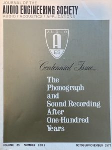
I was reading the AES publication called “The Phonograph and Sound Recording After One-Hundred Years” which was the centennial issue of the Journal of the AES from October / November 1977.
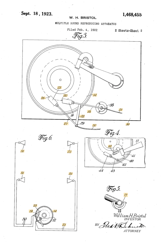
In that issue of the JAES, there is an article called “Record Changers, Turntables, and Tone Arms – A Brief Technical History” by James H. Kogen of Shure Brothers Incorporated, and in that article he mentions US Patent Number 1,468,455 by William H. Bristol of Waterbury, CT, titled “Multiple Sound-Reproducing Apparatus”.
Before I go any further, let’s put the date of this patent in perspective. In 1923, record players existed, but they were wound by hand and ran on clockwork-driven mechanisms. The steel needle was mechanically connected to a diaphragm at the bottom of a horn. There were no electrical parts, since lots of people still didn’t even have electrical wiring in their homes: radios were battery-powered. Yes, electrically-driven loudspeakers existed, but they weren’t something you’d find just anywhere…
In addition, 3- or 2-channel stereo wasn’t invented yet, Blumlein wouldn’t patent a method for encoding two channels on a record until 1931: 8 years in the future…
But, if we look at Bristol’s patent, we see a couple of astonishing things, in my opinion.
If you look at the top figure, you can see the record, sitting on the gramophone (I will not call it a record player or a turntable…). The needle and diaphragm are connected to the base of the horn (seen on the top right of Figure 3, looking very much like my old Telefunken Lido, shown below.
But, below that, on the bottom of Figure 3 are what looks a modern-ish looking tonearm (item number 18) with a second tonearm connected to it (item number 27). Bristol mentions the pickups on these as “electrical transmitters”: this was “bleeding edge” emerging technology at the time.
So, why two pickups? First a little side-story.
Anyone who works with audio upmixers knows that one of the “tricks” that are used is to derive some signal from the incoming playback, delay it, and then send the result to the rear or “surround” loudspeakers. This is a method that has been around for decades, and is very easy to implement these days, since delaying audio in a digital system is just a matter of putting the signal into a memory and playing it out a little later.
Now look at those two tonearms and their pickups. As the record turns, pickup number 20 in Figure 3 will play the signal first, and then, a little later, the same signal will be played by pickup number 26.
Then if you look at Figure 6, you can see that the first signal gets sent to two loudspeakers on the right of the figure (items number 22) and the second signal gets sent to the “surround” loudspeakers on the left (items number 31).
So, here we have an example of a system that was upmixing a surround playback even before 2-channel stereo was invented.
Mind blown…
NB. If you look at Figure 4, you can see that he thought of making the system compatible with the original needle in the horn. This is more obvious in Figures 1 and 2, shown below.