In Part 1, I talked about how an audio signal is quantised, and how the world that the quantised signal lives in is slightly asymmetrical.

Let’s stay in a 3-bit world (to keep things comprehensible on a human scale) and do some recreational quantisation. We’ll start by making a sine wave with a peak amplitude of 1. This means that the total range will be ±1.

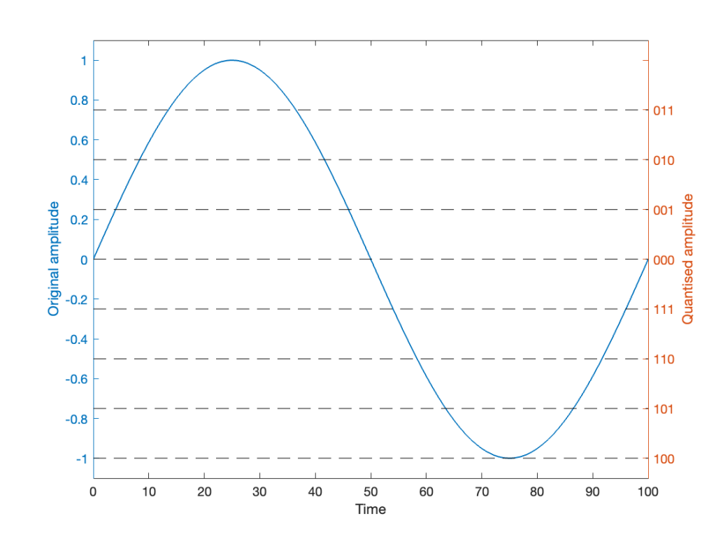
Notice that I put two scales on the plot in Figure 1. On the left, we have the “floating point” amplitude scale. On the right, we have the 8 quantisation levels.

If we are a bit dumb, and we just quantise that sine wave directly, making sure that I’ve aligned the scaling to use ALL possible quantisation values, we get the result in Figure 2.

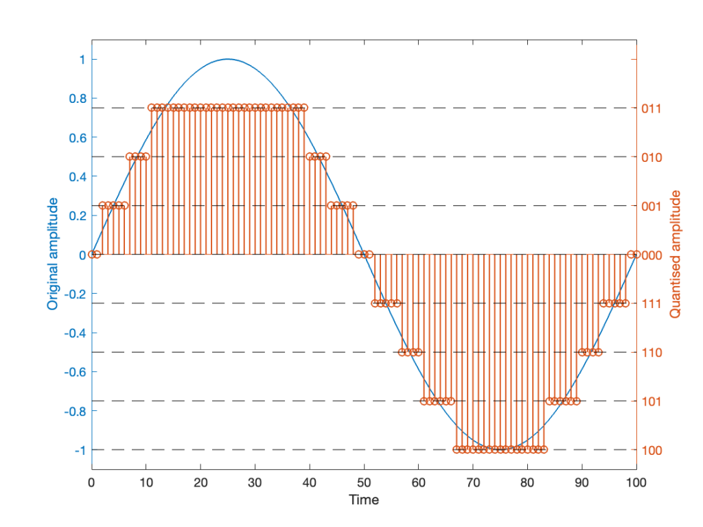
Notice that, because the original signal is symmetrical (with respect to positive and negative amplitudes) but the quantisation steps are not, we wind up getting a different result for the positive values than the negative values. In other words, after quantisation, I’ve clipped the positive peaks of the original signal.

Okay, so this is a dumb way to do this. A slightly less dumb way is to adjust the scaling so that the original wave does not use all possible quantisation values, as shown in Figure 3.

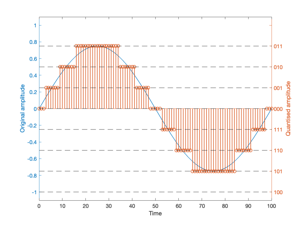
Notice that I’ve set the sine wave to a slightly lower level, so that it rounds to the top-most positive quantisation level, but this means that it doesn’t use the lowest negative quantisation level. If we’re being really picky, I could have made the sine wave just a little higher in amplitude: by 1/2 of a quantisation step, and the quantised result would still not have clipped asymmetrically.

Dither

As you can see in Figures 2 and 3 above, just taking a signal and quantising it generates an error. The more bits you have in the word length, the more quantisation levels you have, and the smaller the error. However, that error will always be correlated with the signal somehow, and as a result, it’s distortion, which is easy to learn to hear.

If, however, we add a little noise to the signal before we quantise it, then we can randomise the error, which changes the error from producing distortion to a constant signal-independent noise floor. Since the noise makes the quantiser appear to be indecisive, we call it dither.

The easiest (and possibly best) way to do this is to create white noise with a triangular probability distribution function and a peak-to-peak amplitude of ± 1 quantisation level. I’ll explain what that last sentence means in Part 3 of this series.

If we do this, then we

• take the signal
• add a little noise to it
• quantise it

and the result might look like Figure 4.

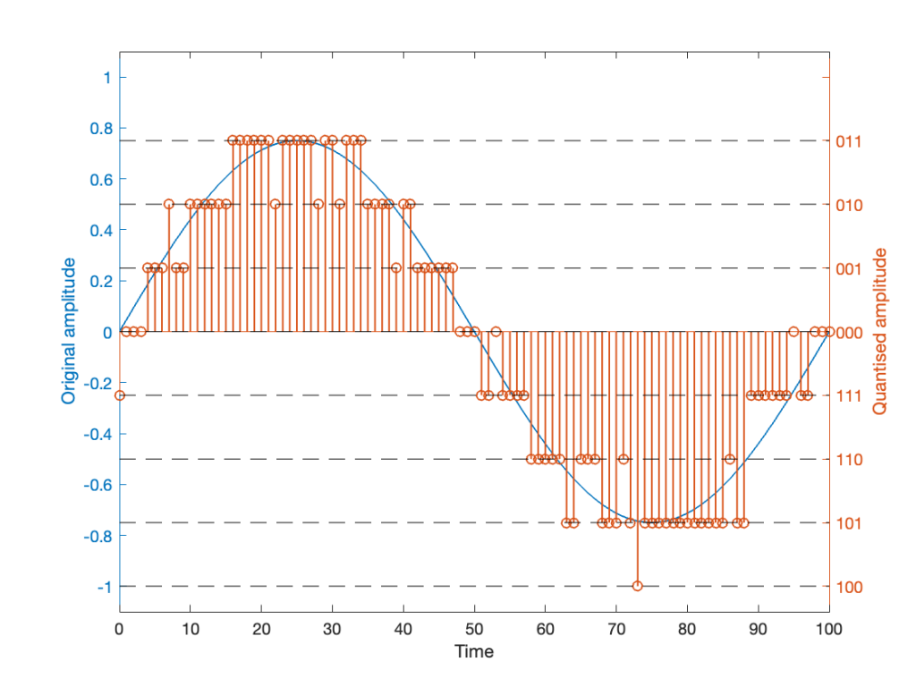
It should be easy to see that we still have quantisation, and also that I’ve added some random element to the signal.

However, let’s look at the mistake I made in Figure 4. The noise that was added to the signal has an amplitude of ±1 quantisation level. So, we should see cases where the signal looks like it should be rounding to the closest level, but it might be either 1 above or 1 below. (For example, take a look at Time = 70, 71, and 72 as an example of this.)

However, take a look around Time = 20 to 30. Notice that the original signal is close to the top quantisation level. This means that, although a negative value in the dither in those samples can bring the quantisation level down, a positive value cannot bring it up because we don’t have any room for it. This will, again, result in a small amount of asymmetrical clipping. This is a VERY small amount. (Remember that, in the real world we’re probably using 2¹⁶ (= 65,536) or 2²⁴ (= 16,777,216) quantisation values, not 2³ (= 8).

So, if we’re going to avoid this clipping, we need to adjust the scaling of the signal once more, as shown in Figure 5.

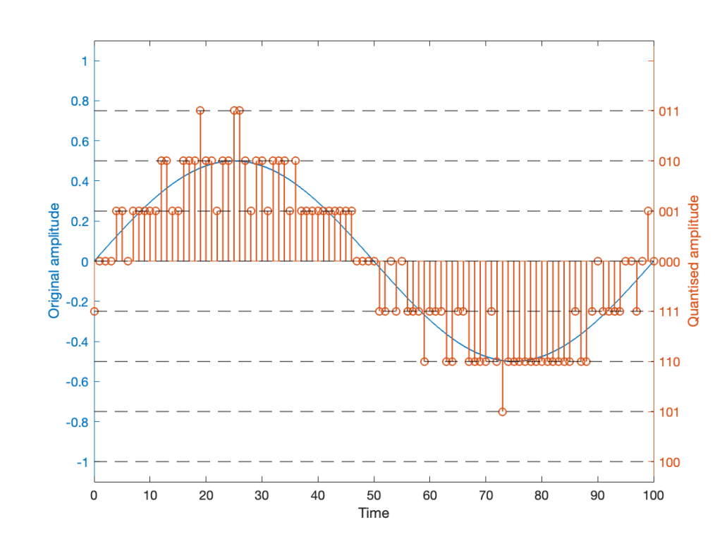
This shows a signal that is scaled so that, without dither, it would round to one level away from the top-most quantisation level. When you add the dither, it can go up to that top quantisation level. (In fact, I happened to use the same dither signal for Figures 4 and 5. The only difference is the scaling of the signal.)

Now, I know that if you’re not used to looking at 3-bit signals, and/or if dither is a new concept, the red signal in Figure 5 might make you a little upset. However (and you have to believe me on this…) this is the correct way to encode digital audio. Just because it looks crazy doesn’t mean that it is.

NB: The math

If you want to make the plots above, here’s a simplified version of the math to try it out. Note: I live in a world where a % symbol precedes a comment.

Some Constants

Bitdepth = 3
Fs = 100 % sampling rate in Hz
Fc = 1 % frequency of the sine wave in Hz
TimeInSamples = [0:Fs] % This will make the TimeInSamples all of the integer values from 0 to Fs (therefore, 1 second of audio)

Figure 1

Signal = sin(2 * pi * Fc/Fs * TimeInSamples)

Figure 2

ScaleUp = 2^(Bitdepth-1)
ScaleDown = 2^(Bitdepth-1)

QuantisedSignal = round(Signal * ScaleUp) / ScaleDown;

% Then apply a clipper to remove the top quantisation level.
% You can do this yourself.

Figure 3

ScaleUp = 2^(Bitdepth-1)-1
ScaleDown = 2^(Bitdepth-1)

QuantisedSignal = round(Signal * ScaleUp) / ScaleDown;

Figure 4

ScaleUp = 2^(Bitdepth-1)-1
ScaleDown = 2^(Bitdepth-1)
TpdfDither = rand(LengthOfSignal) - rand(LengthOfSignal)

QuantisedDitheredSignal = round(Signal * ScaleUp + TpdfDither) / ScaleDown;

% Then apply a clipper to remove the top quantisation level.

Figure 5

ScaleUp = 2^(Bitdepth-1)-2
ScaleDown = 2^(Bitdepth-1)
TpdfDither = rand(LengthOfSignal) - rand(LengthOfSignal)

QuantisedDitheredSignal = round(Signal * ScaleUp + TpdfDither) / ScaleDown;